58. Synthetic Valley Problem
This example is based on a flow and transport problem described in (Hughes et al., 2023). The Synthetic Valley examples represents a developed alluvial valley surrounded by low permeability bedrock. The model includes the Blue Lake and Straight River surface water features (Figure 58.1). The upper two layers represent an unconfined aquifer, the third layer represents a confining unit, and the lower three layers represent the lower aquifer unit. The confining unit only exists in the northern part of the model domain as shown in Figure 58.1.
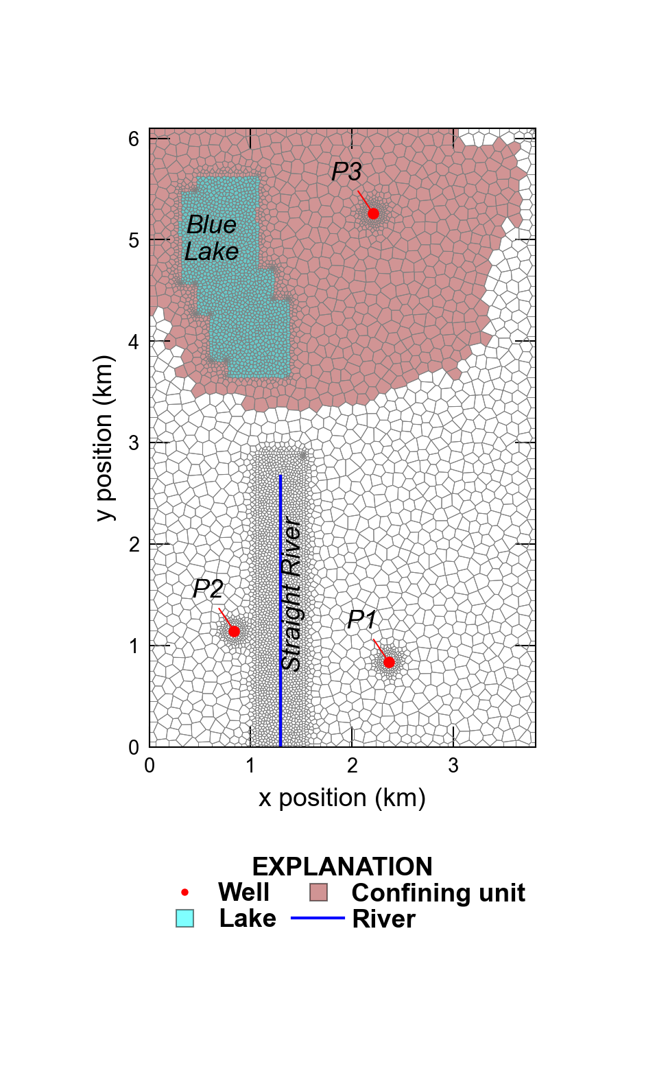
Figure 58.1 Map showing the Voronoi grid used to discretize the model domain and the location of Blue Lake, Straight River, and the areal extent of the confining unit separating the upper and lower aquifer units for the Synthetic Valley example in (Hughes et al., 2023).
58.1. Example description
The 6,096 m x 3,810 m model domain is discretized using a Voronoi grid, with 6,343 active cells per layer, and the discretization by vertices (DISV) package (Figure 58.1). The model grid was refined within Blue Lake, around Straight River, and around pumping wells P1, P2, and P3. The parameters used for this problem are listed in Table 58.1.
Parameter |
Value |
|---|---|
Simulation length (\(d\)) |
10957.5 |
Number of transport time steps |
60 |
Number of layers |
6 |
Rainfall (\(m/d\)) |
0.0025 |
Potential evaporation (\(m/d\)) |
0.0019 |
SFR package length unit conversion |
1.0 |
SFR package time conversion |
86400.0 |
Stream width (\(m\)) |
3.048 |
Stream bed thickness (\(m\)) |
0.3048 |
Stream Manning’s roughness coefficient |
0.030 |
Lake bed leakance (\(1/d\)) |
0.0013 |
LAK package length unit conversion |
1.0 |
LAK package time conversion |
86400.0 |
Drain vertical hydraulic conductivity (\(m/d\)) |
0.03048 |
Drain bed thickness (\(m\)) |
0.3048 |
Drain linear scaling depth (\(m\)) |
0.3048 |
Longitudinal dispersivity (\(m\)) |
75.0 |
Transverse horizontal dispersivity (\(m\)) |
7.5 |
Aquifer porosity (unitless) |
0.2 |
Confining unit porosity (unitless) |
0.4 |
In this example, both groundwater flow (Langevin et al., 2017) and
solute transport (Langevin et al., 2022) are simulated. To better
represent solute transport, the lower aquifer has been discretized into
three layers. Confining units have to be explicitly simulated in
MODFLOW 6, therefore, a total of six layers are simulated. The bottom of
layers 1, 2, 3, and 4 were set to constant values of -1.53, -15.24,
-15.55 and -30.48 m, respectively. Model layer 3 represents the
confining unit and is relatively thin (0.3 m). The IDOMAIN concept
(Langevin et al., 2017) was used to eliminate cells in model layer 3 (by
setting IDOMAIN=-1) where the confining unit does not exist. In
these areas, the thickness of layer 3 was set to zero and IDOMAIN
was set to -1, which marks these cells in layer 3 as “vertical pass
through cells” and results in cells in layer 2 being directly connected
to cells in layer 4.
The bottom of the model (layer 6) is based on (Hill et al., 1998) and the bottom of layer 5 was specified to be half the distance between the bottom of layers 4 and 6. The top of the model was constructed from topographic contours developed for the model that was used as the starting point for (Hill et al., 1998); the top of the model is shown in Figure 58.2A. The top of the model and the bottom of layer 6 were resampled from the data used in (Hill et al., 1998).
The horizontal hydraulic conductivity was discretized into five zones with values of 45.72, 50.29, 60.96, 83.82, and 121.92 m/d; the lowest hydraulic conductivity zone was located south of Blue Lake and the highest hydraulic conductivity zone was located beneath Blue Lake. The vertical hydraulic conductivity in the upper and lower aquifer was specified to be one quarter of the horizontal hydraulic conductivity. The horizontal and vertical hydraulic conductivity in the confining unit was set equal to 9.14\(\times10^{-4}\) m/d. The horizontal and vertical hydraulic conductivity were resampled from the data used in (Hill et al., 1998).
For the groundwater transport model, the porosity, longitudinal dispersivity, and transverse dispersivity were set to values specified in Table 58.1. For the transport model, the Total Variation Diminishing scheme available in the GWT model (Langevin et al., 2022) was used to simulate advection. Molecular diffusion was not represented.
Straight River is simulated using the streamflow routing (SFR) package, and Blue Lake is simulated using the LAK package (Figure 58.1). Straight River was discretized into 108 SFR reaches. The bed thickness and width of each SFR reach were set to values specified in Table 58.1. The leakance for each SFR reach was calculated using the bed thickness, reach width, and reach length in each cell and based on a total Straight River conductance of 50,971.72 m\(^2\)/d. Specified rainfall and potential evaporation rates specified in Table 58.1 were defined for each Straight River reach.
Blue Lake was simulated as a lake on top of the model grid and only had vertical connections to 1,406 cells in the underlying upper aquifer (model layer 1). A bed leakance of 0.0013 1/d was specified for each cell connected to Blue Lake. Specified rainfall and potential evaporation rates specified in Table 58.1 were defined for Blue Lake.
Drain (DRN) cells were specified in each cell in model layer 1 that was not connected to Blue Lake to prevent water levels from exceeding the top of the model. The conductance of each DRN cell was based on the horizontal cell area and the drain bed thickness and vertical hydraulic conductivity specified in Table 58.1. Linear scaling of the drainage conductance was applied to improve model convergence and ranged from 0 m\(^2\)/d when groundwater levels were greater than or equal to 0.3048 m below the top of the model to the specified conductance when groundwater water levels were greater than or equal to the top of the model.
Uniform recharge and potential evapotranspiration rates were specified using the recharge (RCH) and evapotranspiration (EVT) packages, respectively, and were equal to the rates specified in the SFR and LAK packages. The EVT surface was specified to be the top of the model and the EVT extinction depth was specified to be 1 m.
Pumping rates for wells P1, P2, and P3 were -7,600, -7,600, and -1,900 m\(^3\)/d, respectively. All groundwater pumpage was extracted from model layer 6.
Transport was not simulated in the LAK and SFR packages. Instead, a specified concentration condition with a concentration of 1.0 mg/L was specified for Blue Lake. All other stress packages were assumed to have a concentration of 0 mg/L.
An initial head of 11 m was specified for every cell. An initial stage of 3.44 m was specified for Blue Lake. An initial concentration of 0 mg/L was specified for every cell in the transport model.
58.2. Example Results
The groundwater flow model used the Newton-Raphson Formulation with Newton under-relaxation to improve convergence. The groundwater flow and transport models used the Bi-conjugate Stabilized linear accelerator and simple solver settings.
The groundwater flow and transport models were run for a total of 30 years. The groundwater flow model used a single steady-state time step and groundwater flow results were used to run the transport model with a total of 60 time steps with a constant length of 182.625 days.
Simulated heads and vectors of specific discharge in model layer 1 are shown in Figure 58.2B. Specific discharge is greatest on the east side of Blue Lake and in the vicinity of the three pumping wells and Straight River.
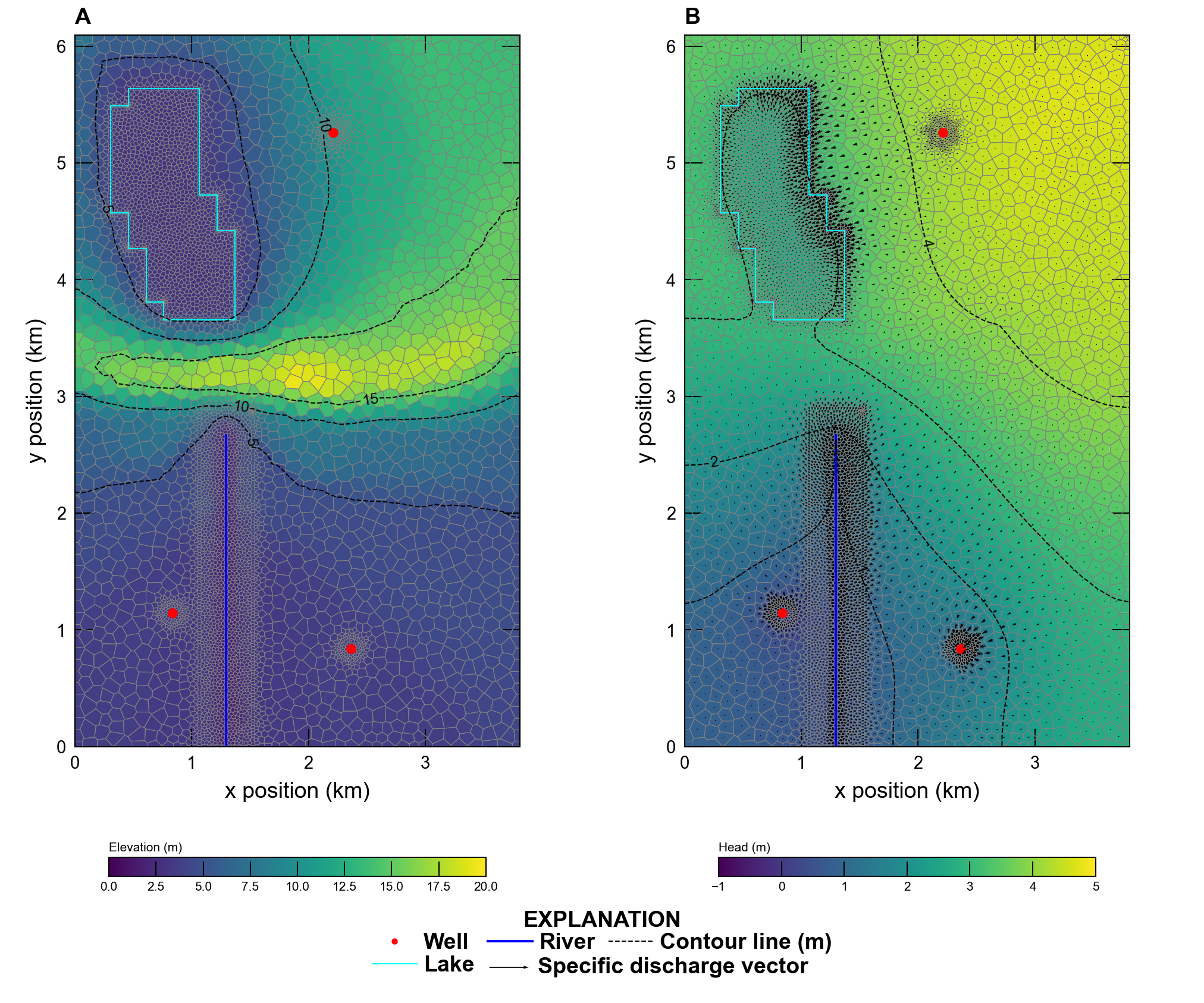
Figure 58.2 Color shaded plot of (A) topography and (B) simulated steady-state heads and specific discharge rates in model layer 1.
Simulated concentrations at the end of 30-years in all six model layers are shown in Figure 58.3. Simulated concentrations are highest beneath Blue Lake in model layer 1 and do not vary much in model layers 1 and 2. Simulated concentrations in model layer 3 are limited to the extent of the confining unit because the remaining cells in the layer are defined to be “vertical pass through cells.” The lateral extent of the solute plume does not vary much south of Blue Lake because of the lack of confinement in these areas.
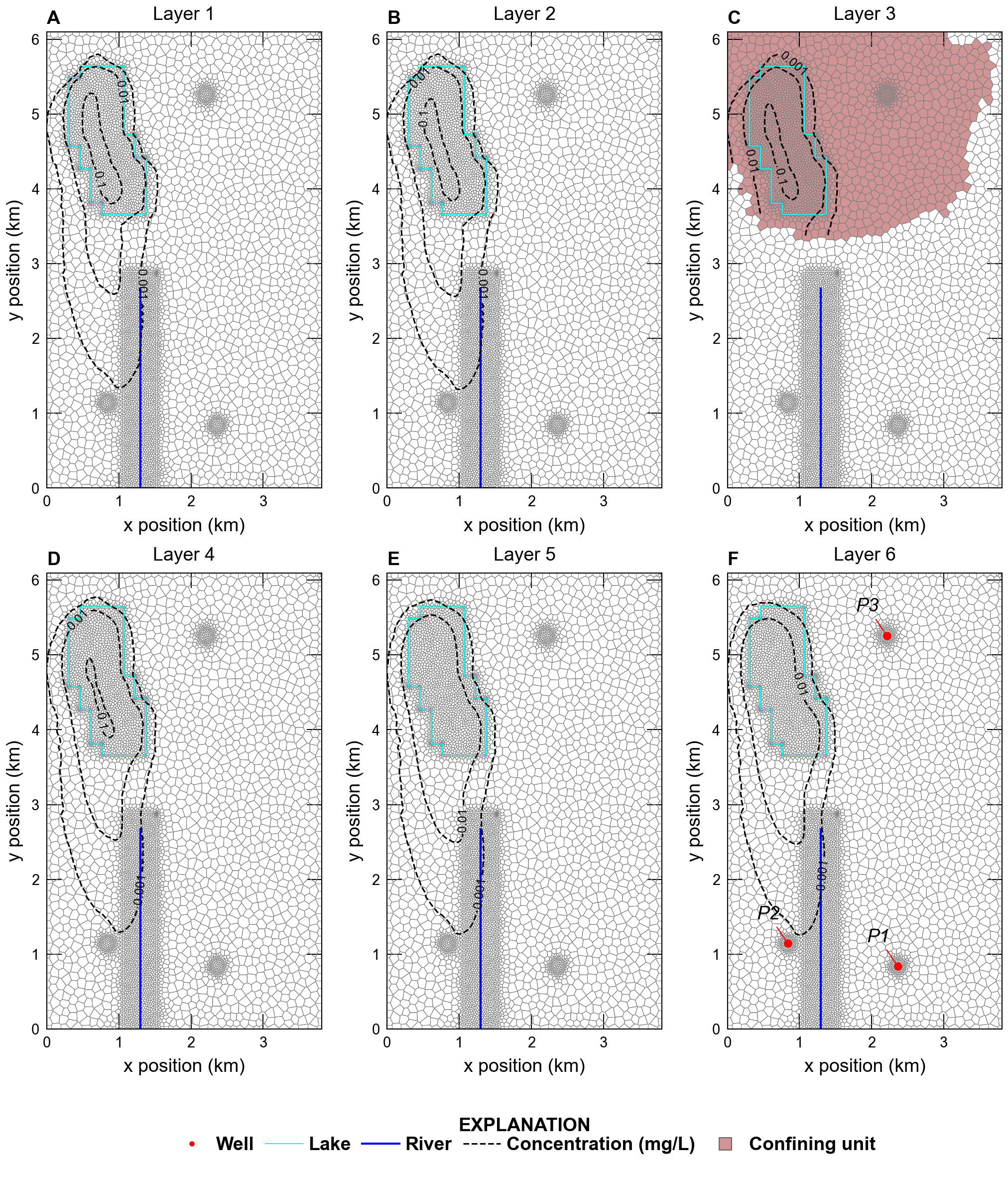
Figure 58.3 Contours of concentrations at the end of 30 years in model layer (A) 1, (B) 2, (C) 3, (D) 4, (E) 5, and (F) 6. The extent of the confining unit in model layer 3 is also shown on (C).
58.3. References Cited
Hill, M. C., Cooley, R. L., & Pollock, D. W. (1998). A controlled experiment in ground water flow model calibration. Groundwater, 36(3), 520–535. https://doi.org/10.1111/j.1745-6584.1998.tb02824.x
Hughes, J. D., Langevin, C. D., Paulinski, S. R., Larsen, J. D., & Brakenhoff, D. (2023). FloPy workflows for creating structured and unstructured MODFLOW models. Groundwater. https://doi.org/10.1111/gwat.13327
Langevin, C. D., Hughes, J. D., Provost, A. M., Banta, E. R., Niswonger, R. G., & Panday, S. (2017). Documentation for the MODFLOW 6 Groundwater Flow (GWF) Model. https://doi.org/10.3133/tm6A55
Langevin, C. D., Provost, A. M., Panday, S., & Hughes, J. D. (2022). Documentation for the MODFLOW 6 groundwater transport (GWT) model. https://doi.org/10.3133/tm6A55
58.4. Jupyter Notebook
The Jupyter notebook used to create the MODFLOW 6 input files for this example and post-process the results is: