14. Lake Package Problem 1
This example is based on problem 1 in the Lake (LAK) Package for MODFLOW-2000 described in (Merritt & Konikow, 2000). The example represents a lake surrounded by a surficial aquifer (Figure 14.1).
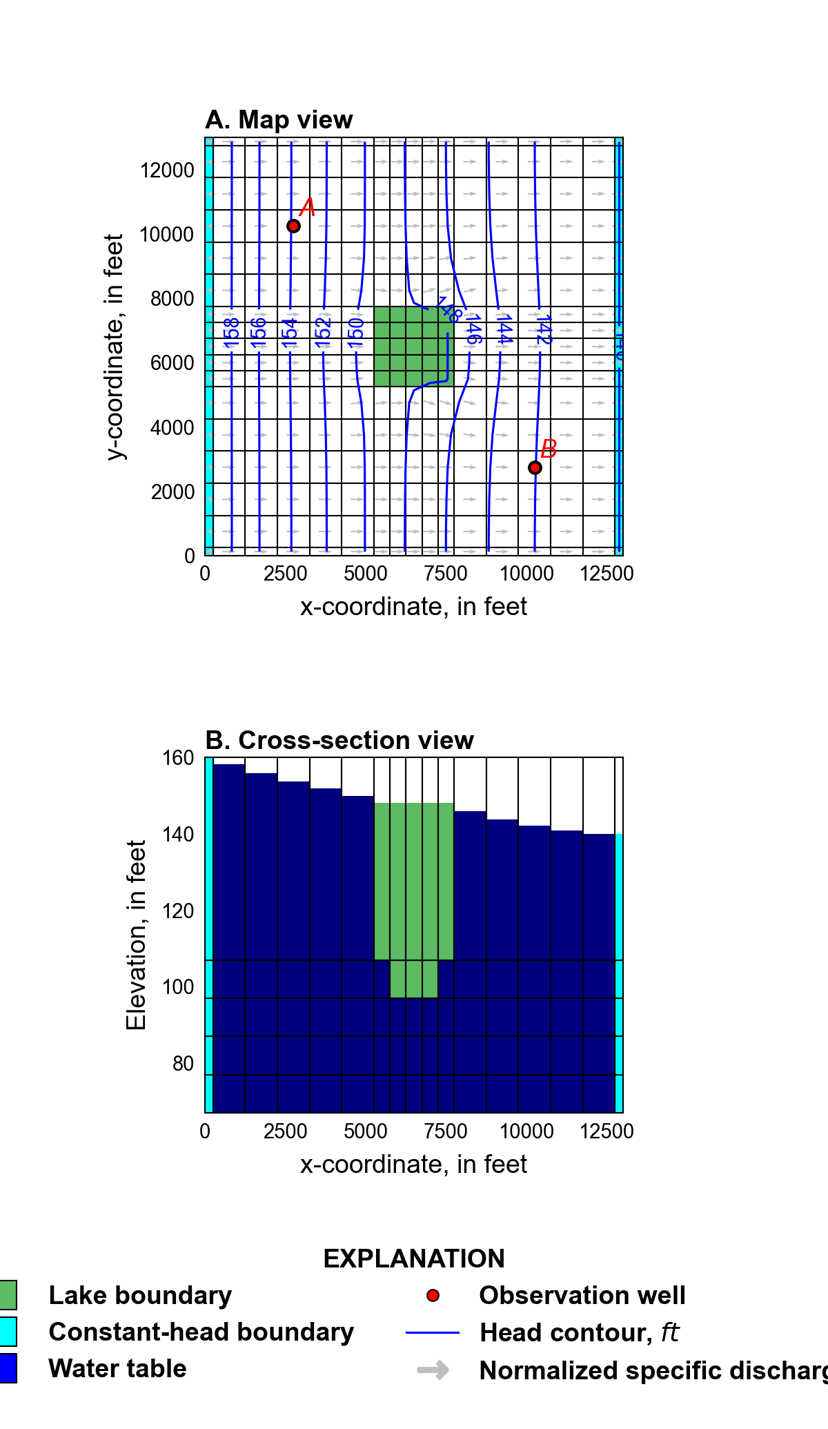
Figure 14.1 Lateral and vertical grid discretization. A. Map view. The location of lake and constant head boundary cells are also shown. Simulated heads and lake stage at the end of stress period 1, normalized specific discharge vectors, and the location of two observation locations are also shown. B. Cross-section view. The location of lake and constant head boundaries are also shown. The water table and lake stage at the end of stress period 1 are also shown.
14.1. Example Description
Model parameters for the example are summarized in
Table 14.1. The model consists of a grid of 17
columns, 17 rows, and 5 layers. The model domain is 13,000 \(ft\) in
the x- and y-directions. The discretization is in the row and column
directions ranges from 250 to 1,000 \(ft\) and is 500 \(ft\) in
the center of the model domain where the lake is located
(Figure 14.1). The top of the model is
specified to be 500 \(ft\) and the bottom of each layer is specified
to be 107, 97, 87, 77, and 67 \(ft\). Groundwater flow was
inactivated in the location of the lake in model layers 1 and 2 by
specifying an IDOMAIN value of zero in these cells.
One transient stress period 5,000 days in length is simulated. The stress period has 100 time steps and uses a time step multiplier equal to 1.02, which results in time step lengths that range 16.01 to 113.74 days.
Parameter |
Value |
|---|---|
Number of periods |
1 |
Number of layers |
5 |
Number of rows |
17 |
Number of columns |
17 |
Top of the model (\(ft\)) |
500.0 |
Bottom elevations (\(ft\)) |
107., 97., 87., 77., 67. |
Starting head (\(ft\)) |
115.0 |
Horizontal hydraulic conductivity (\(ft/d\)) |
30.0 |
Vertical hydraulic conductivity (\(ft/d\)) |
1179., 30., 30., 30., 30. |
Specific storage (\(1/d\)) |
3e-4 |
Specific yield (unitless) |
0.2 |
Constant head on left side of model (\(ft\)) |
160.0 |
Constant head on right side of model (\(ft\)) |
140.0 |
Aereal recharge rate (\(ft/d\)) |
0.0116 |
Maximum evapotranspiration rate (\(ft/d\)) |
0.0141 |
Evapotranspiration extinction depth (\(ft\)) |
15.0 |
Starting lake stage (\(ft\)) |
110.0 |
Lake evaporation rate (\(ft/d\)) |
0.0103 |
Lakebed leakance (\(1/d\)) |
0.1 |
The horizontal and vertical hydraulic conductivity is 30 \(ft/day\) except for the vertical hydraulic conductivity of layer 1 which was specified to be 1,179 \(ft/d\). A constant specific storage value of \(3 \times 10^{-4}\) (\(1/day\)) and specific yield of 0.2 (unitless) were specified. All model layers were specified to convert between confined and unconfined conditions. An initial head of 115 \(ft\) was specified in all model layers.
Flow into the system is from infiltration from precipitation and was represented using the recharge (RCH) package and a constant recharge rate of 0.0116 \(ft/d\). Flow out of the model is from groundwater evapotranspiration represented by evapotranspiration (EVT) package cells. Groundwater evapotranspiration occurs where depth to water is within 15 \(ft\) of land surface, has a maximum rate of 0.0141 \(ft/d\) at land surface. The evapotranspiration surface, the elevation in the aquifer below which evapotranspiration is assumed to decline linearly, is represented as linearly sloping from 160 \(ft\) on the left side of the model to 140 \(ft\) on the right side of the model, except in the lake area, where the elevation is specified as 3 \(ft\) below the lakebed, which is equal to 2 \(ft\) below the layer bottom elevation. This means that in the possible case of lake drying, land-surface evapotranspiration from the water table under the dry lakebed is at the maximum rate if the water table is not deeper than 3 \(ft\) below the lakebed. Away from the lake, the evapotranspiration surface is an implicit representation of land surface, since the latter is normally equal to or slightly above the evapotranspiration surface. Constant head boundary cells were added in column 1 and column 17 in all rows and layers; constant heads are specified to be 160 and 140 \(ft\) on the left and right sides of the model, respectively.
The lake is located in the center of the model domain in model layers 1 and 2 and has an initial stage of 110 \(ft\). The lake is connected horizontally to the aquifer in model layers 1 and 2 and vertically to cells in model layer 2 and 3 that directly underly the lake. A lakebed leakance value of 0.1 \(1/d\) was specified for all lake connections to the aquifer. The connection length for horizontal lake connections were calculated from grid dimensions and are 500 \(ft\) in layer 1 and 250 \(ft\) in layer 2; the connection width for horizontal connections was 500 \(ft\). Rainfall and evaporation rates equal to 0.0116 and 0.0103 \(ft/d\) are specified for the lake, respectively.
The model uses the Newton-Raphson Formulation. The simple complexity Iterative Model Solver option and preconditioned bi-conjugate gradient stabilized linear accelerator is also used.
14.2. Example Results
Simulated results at the end of the stress period are shown in Figure 14.1. Transient results for the lake stage and groundwater heads at two aquifer locations are shown in Figure 14.2. Both water-table elevations and the lake stage converge asymptotically to equilibrium values. The water-table elevations approximately converge in about 1,000 days and the lake stage in about 2,000 days of simulation time.
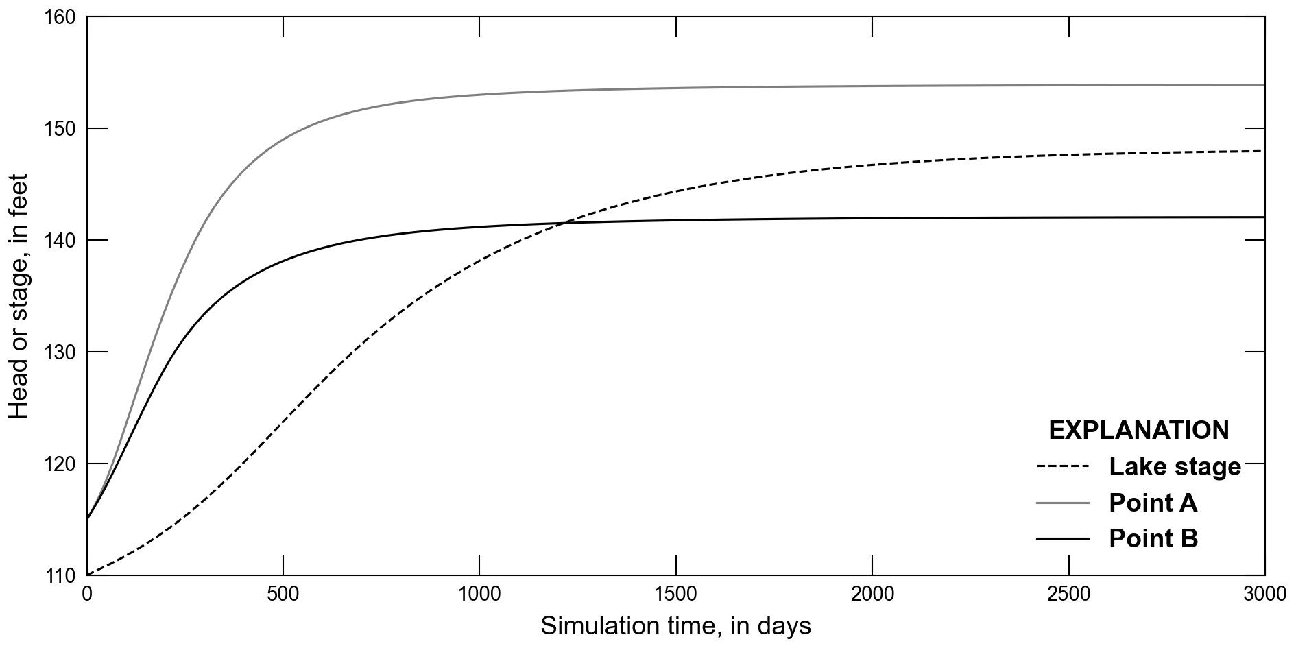
Figure 14.2 Selected heads in the aquifer and the lake stage. The location of points A and B are shown in Figure 14.1.
14.3. References Cited
Merritt, M. L., & Konikow, L. F. (2000). Documentation of a computer program to simulate lake-aquifer interaction using the MODFLOW ground-water flow model and the MOC3D solute-transport model. Retrieved from https://pubs.er.usgs.gov/publication/wri004167
14.4. Jupyter Notebook
The Jupyter notebook used to create the MODFLOW 6 input files for this example and post-process the results is: