46. MT3DMS Problem 10
This example problem describes an actual field problem (Zheng & Wang, 1999). While the original discussion of this problem compared various MT3MDS solution schemes and evaluated the effectiveness of MT3DMS for solving real-world problems, the current goal is much more modest: to compare the MODFLOW 6 transport solution against the MT3DMS solution.
46.1. Example description
The geological setting for this final problem from (Zheng & Wang, 1999) is roughly shown in Figure 46.1. An unconfined aquifer beneath a spill site is approximately divided into an upper and lower zone with hydraulic conductivities of 60 and 520 \(ft/day\), respectively. Each zone is represented by two 25 \(ft\) uniformlyh thick layers, for a total of 4 layers. Each layer is comprised of 61 rows and 40 columns with variable row and column widths. The highest level of grid refinement exists near the detailed study site containing the bulk of the contaminant plume. In this area, row and column widths are 50 \(\times\) 50 \(ft\) (area denoted by ABCD in Figure 46.1). Outside this area, cell lengths and widths progressively increase toward the model boundary. A no-flow no-flux boundary conditions is applied to the bottom boundary while specified head boundaries are used on all four sides. Heads along the sides of the model domain estable a regional flow gradient of \(5 \times 10^{-4}\) from east to west and \(1 \times 10^{-3}\) from north to south. Mass may leave the model domain with the regional flow gradient, but does so at the computed concentration of the groundwater. Water that enters the model domain via the regional flow gradient does so with a concentration of 0.0. However, model boundaries are intentionally set far enough away from the area of concern so that their effect on the flow and transport simulation is minimized. A constant recharge rate of 5 \(in/yr\) is applied to the surface of the model. A uniform porosity of 0.30 is applied to the entire model. Owing to the presence of organic contaminants within the groundwater, including 1,2-dichloroethane (1,2-DCA), chemical reactions are simulated using an equilibrium-controlled linear sorption isotherm. Reactive parameters are specified such that the retardation term equals 2. The initial concentration of 1,2-DCA for layer 1 is shown in Figure 46.2A. The initial concentration of 1,2-DCA in layer 2 is 20 percent of the layer 1 initial concentration. Layers 3 and 4 start out with no contaminant. The location of extraction wells are given by the black squares in Figure 46.2. The extraction wells are used to pump-and-treat contaminated goundwater. The total specified extraction rate among all wells is \(4.25 \times 10^3 m^3/day\) which occurs from layer 3. The Additional model parameter values are listed in Table 46.1.
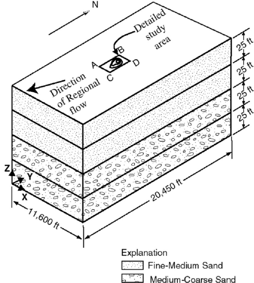
Figure 46.1 MT3DMS test problem 10 showing the numerical model configuration. Image not to scale. (11,600 ft = 3.535.68 m; 20,450 ft = 6,233 m; 25 ft = 7.62 m)
Parameter |
Value |
|---|---|
Number of layers |
4 |
Number of rows |
61 |
Number of columns |
40 |
Column width (\(ft\)) |
varies |
Row width (\(ft\)) |
varies |
Layer thickness (\(ft\)) |
25.0 |
Top of the model (\(ft\)) |
780.0 |
Saturated thickness (\(ft\)) |
100.0 |
Horiz. hyd. conductivity of layers 1 and 2 (\(ft/day\)) |
60.0 |
Horiz. hyd. conductivity of layers 3 and 4 (\(ft/day\)) |
520.0 |
Ratio of vertical to horizontal hydraulic conductivity |
0.1 |
Recharge rate (\(in/yr\)) |
5.0 |
Concentration of recharge (\(ppm\)) |
0.0 |
Porosity |
0.3 |
Longitudinal dispersivity (\(ft\)) |
10.0 |
Ratio of horizontal transverse dispersivity to longitudinal dispersivity |
0.2 |
Ratio of vertical transverse dispersivity to longitudinal dispersivity |
0.2 |
Aquifer bulk density (\(g/cm^3\)) |
1.7 |
Distribution coefficient (\(cm^3/g\)) |
0.176 |
Simulation time (\(days\)) |
1000.0 |
46.2. Example results
The calculated concentration fields are shown for layer 3 at 500, 750, and 1,00 days in Figure 46.1B-D, respectively. Both models use their finite-difference solutions and therefore do no invoke their respective TVD scheme. Relatively good agreement between the two simulations is achieved in the lower (southerly) portion of the model for all 3 simulation times displayed. In the upper (northerly) portion of the model, however, several cells separate the isoconcentration contours.
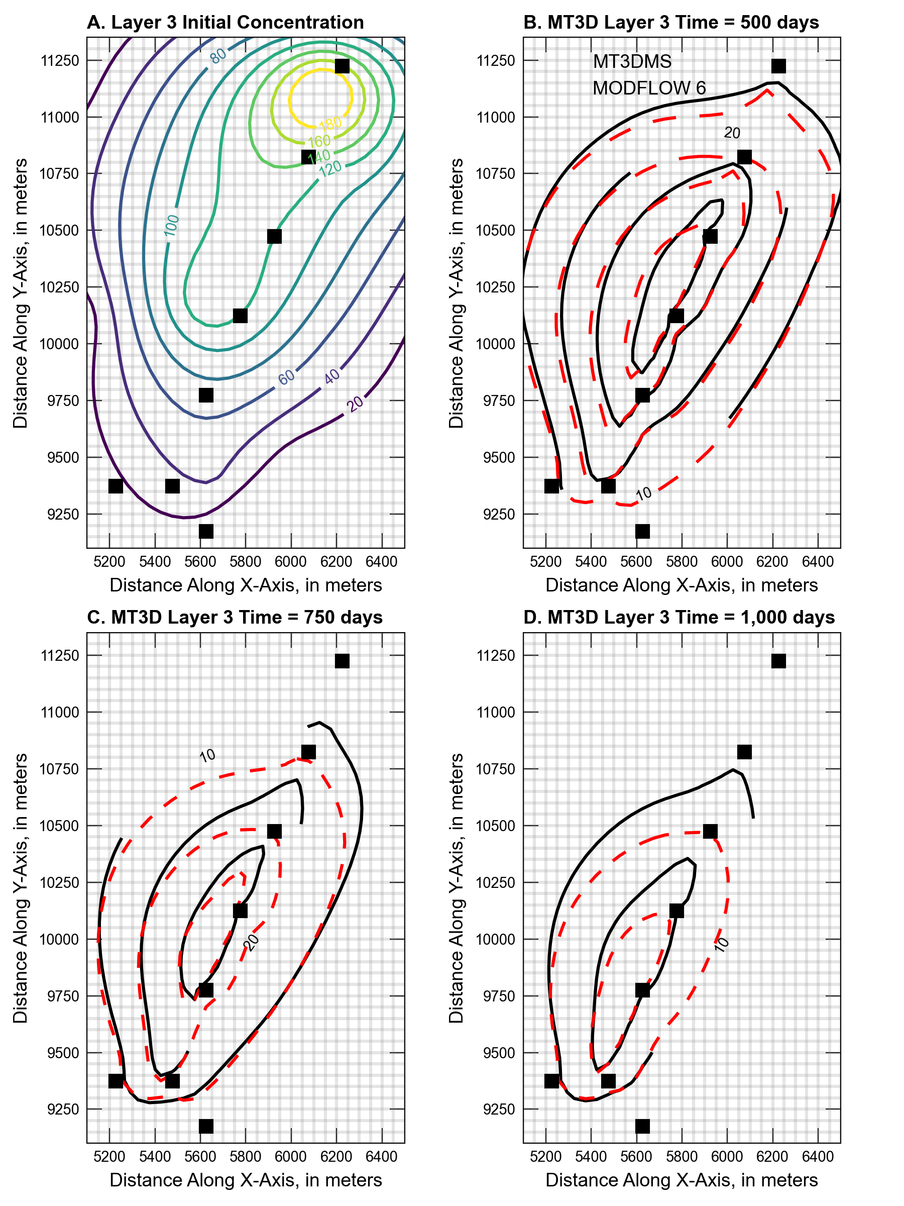
Figure 46.2 (A) Initial and simulated contaminant plume concentrations as calculated by MT3DMS and MODFLOW 6 after (B) 500 days, (C) 750 days, and (D) 1,000 days.
46.3. References Cited
Zheng, C., & Wang, P. P. (1999). MT3DMS—a modular three-dimensional multi-species transport model for simulation of advection, dispersion and chemical reactions of contaminants in groundwater systems; documentation and user’s guide.
46.4. Jupyter Notebook
The Jupyter notebook used to create the MODFLOW 6 input files for this example and post-process the results is: