37. MT3DMS Problem 1
Section 7 of (Zheng & Wang, 1999) details a number of test problems that verify the accuracy of MT3DMS. The first problem presented, titled “one-dimensional transport in a uniform flow field,” compared MT3DMS solutions to analytical solutions given by (Van Genuchten & Alves, 1982). For verifying the accuracy of transport calculations within MODFLOW6, the transport solutions calculated by MT3DMS serve as the benchmark to which the MODFLOW 6 solution is compared. The first 1-dimensional simulation solves for advection only. The second model permutation uses both advection and dispersion to verify MODFLOW 6 results. Next, the accuracy of MODFLOW 6 is verified when advection, dispersion, and some simple checmial reactions represented with sorption processes are used. The fourth and final model permutation adds solute decay to the previous model setup. As of the first release of MODFLOW 6 with transport capabilities, a linear isotherm is the only option available for simulating sorption. Arbitrary values of bulk density and distribution coefficient are uniformly applied to the entire model domain to achieve the indicated retardation factor. The following table summarizes how the four simulations incrementally increase model complexity.
Scenario |
Scenario Name |
Parameter |
Value |
|---|---|---|---|
1 |
ex-gwt-mt3dms-p01a |
dispersivity (\(m\)) |
0.0 |
retardation (unitless) |
1.0 |
||
decay (\(d^{-1}\)) |
0.0 |
||
2 |
ex-gwt-mt3dms-p01b |
dispersivity (\(m\)) |
10.0 |
retardation (unitless) |
1.0 |
||
decay (\(d^{-1}\)) |
0.0 |
||
3 |
ex-gwt-mt3dms-p01c |
dispersivity (\(m\)) |
10.0 |
retardation (unitless) |
5.0 |
||
decay (\(d^{-1}\)) |
0.0 |
||
4 |
ex-gwt-mt3dms-p01d |
dispersivity (\(m\)) |
10.0 |
retardation (unitless) |
5.0 |
||
decay (\(d^{-1}\)) |
0.002 |
37.1. Example description
All four model scenarios have 101 columns, 1 row, and 1 layer. The first and last columns use constant-head boundaries to simulate steady flow in confined conditions. Because the analytical solution assumes an infinite 1-dimensional flow field, the last column is set far enough from the source to avoid interfering with the final solution after 2,000 days. Initially, the model domain is devoid of solute; however, the first column uses a constant concentration boundary condition to ensure that water entering the simulation has a unit concentration of 1. Additional model parameters are shown in Table 37.2.
For these simulations, all MODFLOW 6 and MT3DMS simulations use the upstream-weighted finite-difference scheme for representing solute advection.
Parameter |
Value |
|---|---|
Number of periods |
1 |
Number of layers |
1 |
Number of columns |
101 |
Number of rows |
1 |
Column width (\(m\)) |
10.0 |
Row width (\(m\)) |
1.0 |
Top of the model (\(m\)) |
0.0 |
Layer bottom elevations (\(m\)) |
–1.0 |
Porosity |
0.25 |
Simulation time (\(days\)) |
2000 |
Horizontal hydraulic conductivity (\(m/d\)) |
1.0 |
37.2. Example Results
The comparison of the MT3DMS and MODFLOW 6 solutions for problem 1a, an advection dominated problem, represents an end-member test as the migrating concentration front is sharp. Results for both the MODFLOW 6 and MT3DMS results are shown in Figure 37.1. The grid Peclet number is infinity for this problem (\(P_e\) = \(v\Delta x/D_{xx}\) = \(\Delta x\)/\(\alpha_L\) = \(\infty\)). Though not shown here, this advection-only problem can also be represented with the TVD schemes in both MODFLOW 6 and MT3DMS. For this particular problem, the TVD scheme in MT3DMS (called the ULTIMATE scheme) is better able to minimize numerical dispersion than the TVD scheme in MODFLOW 6.
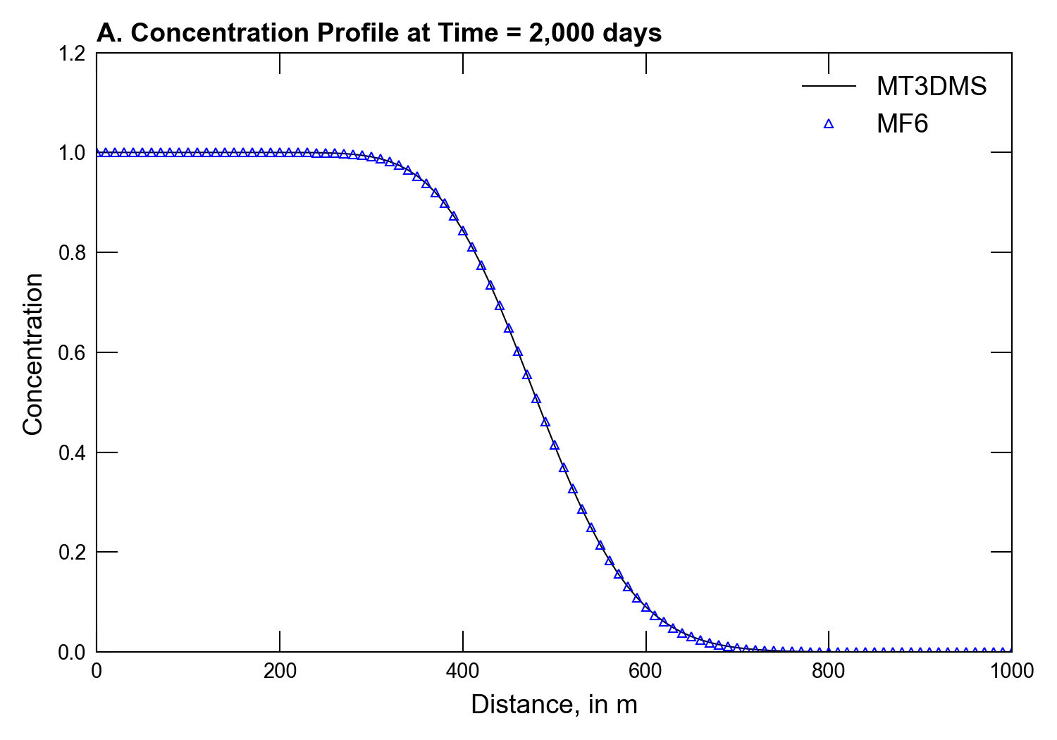
Figure 37.1 Comparison of the MT3DMS and MODFLOW 6 numerical solutions for a one-dimensional advection dominated test problem. The analytical solution for this problem was originally given in (Van Genuchten & Alves, 1982) and is not shown here
A comparison of MT3DMS and MODFLOW 6 for scenario 2 in the MT3DMS manual represents a more common situation whereby dispersion acts to spread or smooth the advancing concentration front. For this problem, the dispersion term \(\alpha_L\) is set equal to the length of the grid cell in the direction of flow, 10 cm, resulting in a Peclet number equal to one (\(P_e\) = \(v\Delta x/D_{xx} = 10/10 = 1\)). Owing to the presence of dispersion, the finite-difference solutions employed by both MT3DMS and MODFLOW 6 for this problem are more accurate, and as a result are in closer agreement (Figure 37.2).
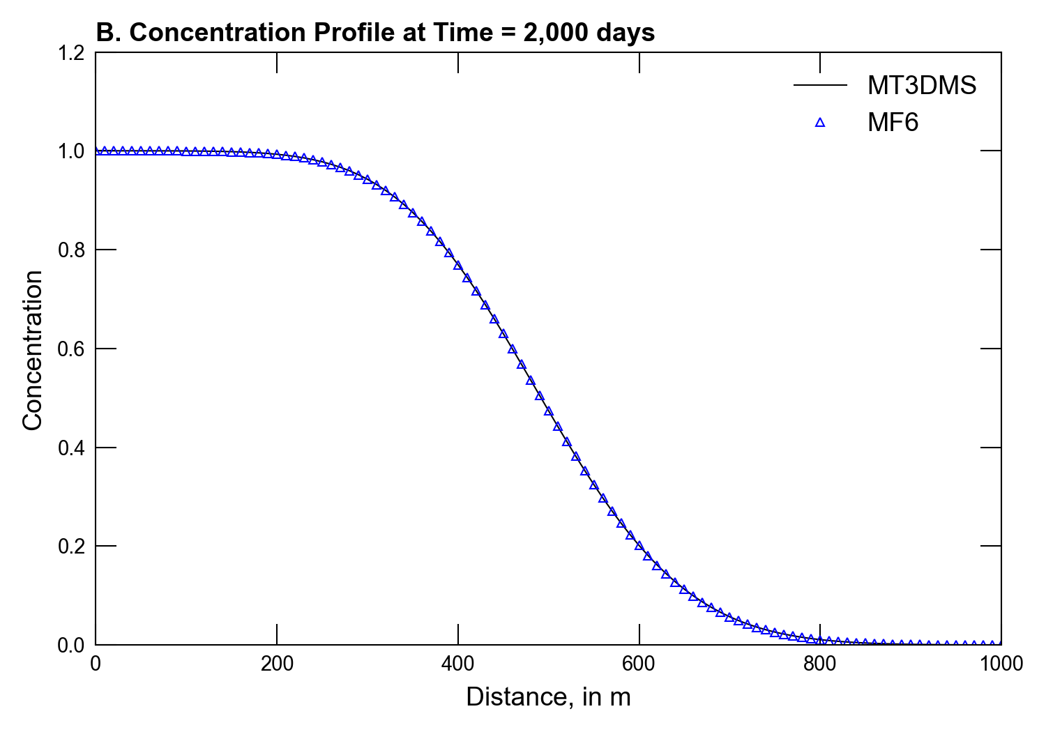
Figure 37.2 Comparison of the MT3DMS and MODFLOW 6 numerical solutions for a one-dimensional test problem with dispersion (\(\alpha_L\) = 10 \(cm\)). The analytical solution for this problem was originally given in (Van Genuchten & Alves, 1982) and is not shown here
The third comparison for the one-dimensional transport in a steady flow field includes uses the same dispersion specified for the second scenario, but adds retardation. For this problem, retardation slows the advance of the migrating concentration front by simulating sorption of the dissolved solute onto the matrix material through which the fluid is moving. In this way, dissolved mass is transferred from the aqueous phase to the solid phase. Appropriate reaction package parameter values are determined for obtaining the specified retardation (5.0) within the code. Figure 37.3 shows a close match between MT3DMS and MODFLOW 6. In addition, Figure 37.3 also shows that after 2,000 days, the concentration front did not advance as far as shown in Figure 37.2.
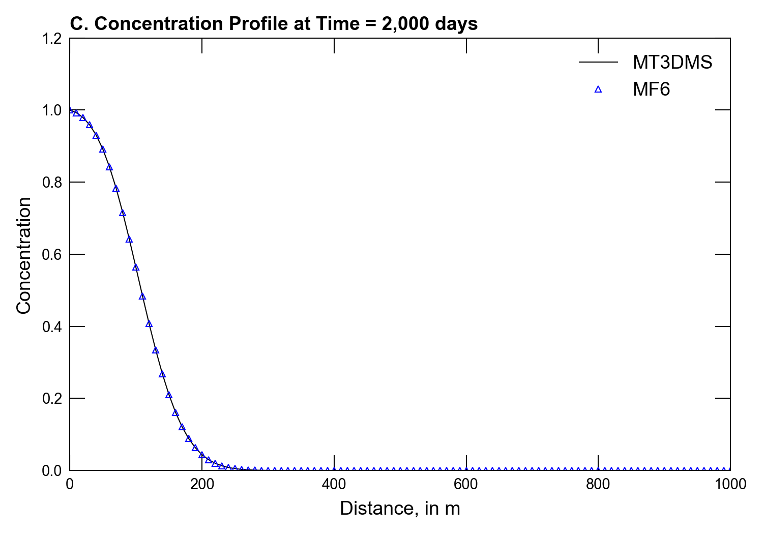
Figure 37.3 Comparison of the MT3DMS and MODFLOW 6 numerical solutions for a one-dimensional test problem with dispersion (\(\alpha_L\) = 10 \(cm\)) and retardation (\(R\) = \(5.0\)). The analytical solution for this problem was originally given in (Van Genuchten & Alves, 1982) and is not shown here
The final comparison for the fourth scenario of problem 1 adds decay to the dispersion and retardation simulated in the third scenario. For this case, decay represents the irreversible loss of mass from both the aqueous and sorbed phases, further stunting the advance of the migrating concentration front Figure 37.4.
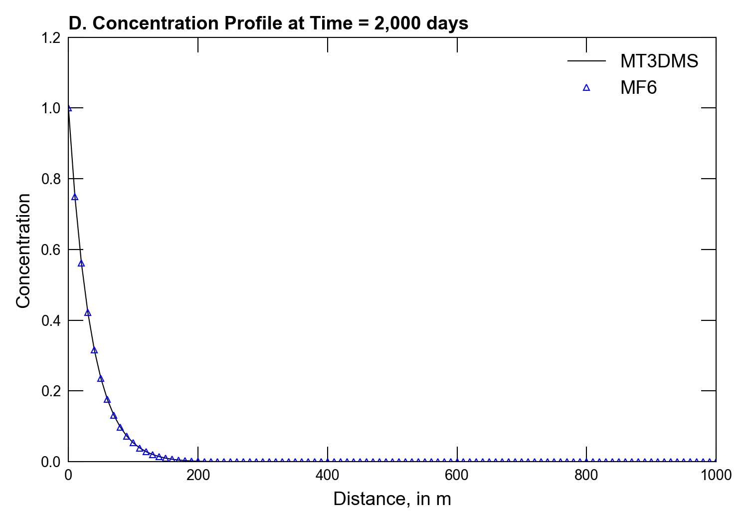
Figure 37.4 Comparison of the MT3DMS and MODFLOW 6 numerical solutions for a one-dimensional test problem with dispersion (\(\alpha_L\) = 10 \(cm\)), retardation (\(R\) = \(5.0\)) and decay (\(\lambda\) = 0.002 \(d^{-1}\)). The analytical solution for this problem was originally given in (Van Genuchten & Alves, 1982) and is not shown here
37.3. References Cited
Van Genuchten, M. T., & Alves, W. J. (1982). Analytical solutions of the one-dimensional convective-dispersive solute transport equation. Retrieved from https://naldc.nal.usda.gov/download/CAT82780278/PDF
Zheng, C., & Wang, P. P. (1999). MT3DMS—a modular three-dimensional multi-species transport model for simulation of advection, dispersion and chemical reactions of contaminants in groundwater systems; documentation and user’s guide.
37.4. Jupyter Notebook
The Jupyter notebook used to create the MODFLOW 6 input files for this example and post-process the results is: