22. Groundwater Whirls
This problem is based on the first whirl problem described by (Provost et al., 2017). Using steady-state groundwater flow simulations, Hemker et al. (2004) have shown that “spiraling flow lines occur in layered aquifers that have different anisotropic horizontal hydraulic conductivities in adjacent layers.” They refer to such spiraling flow lines as “groundwater whirls.” This example demonstrates the use of the XT3D option to implement anisotropy that induces groundwater whirls in a highly idealized two-aquifer system.
22.1. Example Description
The model domain (Figure 22.1) is a box that is 5,100 m by 1,000 m horizontally and 1,000 m thick, discretized into a regular grid of 10 rows, 51 columns, and 10 layers. The top five model layers form the top aquifer, and the bottom five model layers form the bottom aquifer. All cells are confined. Aquifer properties are homogeneous within each aquifer but differ between the aquifers. Groundwater recharges one end of the box at a total rate of 1 m\(^{3}\)/d, distributed equally among 100 cells, and is removed from the opposite end of the box at the same rate, also distributed equally among 100 cells. There is a single steady-state stress period with a length of 1 day. Model parameters are listed in Table 22.1. An initial head of 0 \(m\) was specified for the model. The value is not important as the model is steady state.
The simulation reported, which corresponds to the first whirl problem presented by (Provost et al., 2017) here uses 10:1 horizontal anisotropy (\(K11 = K33 =\) 1 m/d, \(K22 =\) 0.1 m/d) rotated 45 degrees counterclockwise from the \(x\) axis in the top aquifer and 45 degrees clockwise from the \(x\) axis in the bottom aquifer.
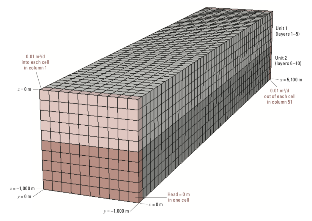
Figure 22.1 Diagram showing the model domain for the whirl problem, which consists of a three-dimensional box with two hydrogeologic units (light and dark shading). Groundwater is injected into one end of the box (column 1, pink shading) at a rate of 0.01 cubic meters per day (\(m^3/d\)) into each cell and is removed from the opposite end of the box (column 51, pink shading) at a rate of 0.01 \(m^3/d\) from each cell. From (Provost et al., 2017).
Parameter |
Value |
|---|---|
Number of periods |
1 |
Number of layers |
10 |
Number of rows |
10 |
Number of columns |
51 |
Spacing along rows (\(m\)) |
100.0 |
Spacing along columns (\(m\)) |
100.0 |
Top of the model (\(m\)) |
0.0 |
Layer bottom elevations (\(m\)) |
–100, –200, –300, –400, –500, –600, –700, –800, –900, –1000 |
Starting head (\(m\)) |
0.0 |
Cell conversion type |
0 |
Hydraulic conductivity in the 11 direction (\(m/d\)) |
1.0 |
Hydraulic conductivity in the 22 direction (\(m/d\)) |
0.1 |
Hydraulic conductivity in the 33 direction (\(m/d\)) |
1.0 |
Rotation of the hydraulic conductivity ellipsoid in the x-y plane |
45, 45, 45, 45, 45, –45, –45, –45, –45, –45 |
Inflow rate (\(m^3/d\)) |
0.01 |
22.2. Example Results
The whirl flow pattern is shown by plotting specific discharge vectors in cross section for column 1 (Figure 22.2).
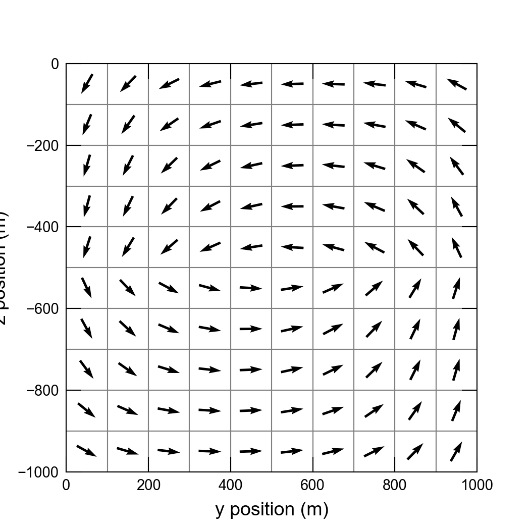
Figure 22.2 Cross section showing vectors of specific discharge for column 1 of the groundwater whirl problem. Vectors show the swirling flow pattern caused by the contrast in the hydraulic conductivity ellipsoid which occurs and the interface between model layer 5 and model layer 6.
22.3. References Cited
Hemker, K., Berg, E. van den, & Bakker, M. (2004). Ground water whirls. Ground Water, 42(2), 234–242. https://doi.org/10.1111/j.1745-6584.2004.tb02670.x
Provost, A. M., Langevin, C. D., & Hughes, J. D. (2017). Documentation for the “XT3D” Option in the Node Property Flow (NPF) Package of MODFLOW 6. https://doi.org/10.3133/tm6A56
22.4. Jupyter Notebook
The Jupyter notebook used to create the MODFLOW 6 input files for this example and post-process the results is: