15. Lake Package Problem 2
This example is based on problem 2 in the Lake (LAK) Package for MODFLOW-2000 described in (Merritt & Konikow, 2000). The example represents a two lakes connected by a stream surrounded by a surficial aquifer (Figure 15.1). The problem has been modified to use the Newton-Raphson Formulation instead of the Standard Conductance Formulation with Node Property Flow (NPF) Package rewetting option.
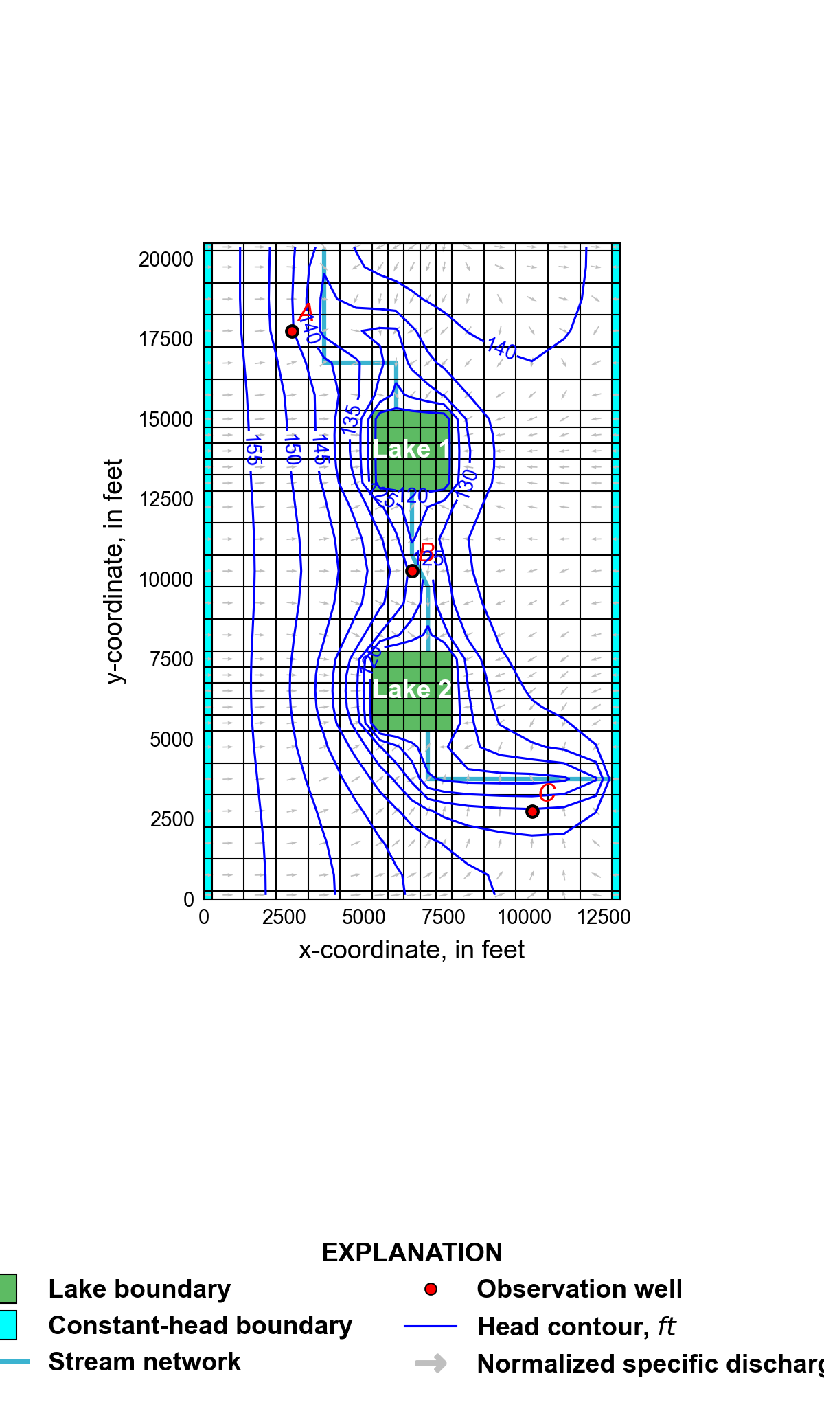
Figure 15.1 Lateral grid discretization. The location of lake and constant head boundary cells are also shown. Simulated heads and lake stage at the end of stress period 1, normalized specific discharge vectors, and the location of three observation locations are also shown.
15.1. Example Description
Model parameters for the example are summarized in
Table 15.1. The model consists of a grid of 17
columns, 27 rows, and 5 layers. The model domain is 13,000 and 20,500
\(ft\) in the x- and y-directions, respectively. The discretization
is in the row and column directions ranges from 250 to 1,000 \(ft\)
and is 500 \(ft\) where the lakes are located
(Figure 15.1). The top of the model is
specified to be 200 \(ft\) and the bottom of each layer is specified
to be 102, 97, 87, 77, and 67 \(ft\). Groundwater flow was
inactivated in the location of the lakes in model layers 1 and 2 by
specifying an IDOMAIN value of zero in these cells.
One transient stress period 1,500 days in length is simulated. The stress period has 200 time steps and uses a time step multiplier equal to 1.005, which results in time step lengths that range 4.40 to 11.82 days.
Parameter |
Value |
|---|---|
Number of periods |
1 |
Number of layers |
5 |
Number of rows |
27 |
Number of columns |
17 |
Top of the model (\(ft\)) |
200.0 |
Bottom elevations (\(ft\)) |
102., 97., 87., 77., 67. |
Starting head (\(ft\)) |
115.0 |
Horizontal hydraulic conductivity (\(ft/d\)) |
30.0 |
Vertical hydraulic conductivity (\(ft/d\)) |
30.0 |
Specific storage (\(1/d\)) |
3e-4 |
Specific yield (unitless) |
0.2 |
Constant head on left side of model (\(ft\)) |
160.0 |
Constant head on right side of model (\(ft\)) |
140.0 |
Aereal recharge rate (\(ft/d\)) |
0.0116 |
Maximum evapotranspiration rate (\(ft/d\)) |
0.0141 |
Evapotranspiration extinction depth (\(ft\)) |
15.0 |
Starting lake stage (\(ft\)) |
130.0 |
Lake evaporation rate (\(ft/d\)) |
0.0103 |
Lakebed leakance (\(1/d\)) |
0.1 |
The horizontal and vertical hydraulic conductivity is 30 \(ft/d\). A constant specific storage value of \(3 \times 10^{-4}\) (\(1/day\)) and specific yield of 0.2 (unitless) were specified. All model layers were specified to convert between confined and unconfined conditions. An initial head of 115 \(ft\) was specified in all model layers.
Flow into the system is from infiltration from precipitation and was represented using the recharge (RCH) package and a constant recharge rate of 0.0116 \(ft/d\). Flow out of the model is from groundwater evapotranspiration represented by evapotranspiration (EVT) package cells. Groundwater evapotranspiration occurs where depth to water is within 15 \(ft\) of land surface, has a maximum rate of 0.0141 \(ft/d\) at land surface. The evapotranspiration surface, the elevation in the aquifer below which evapotranspiration is assumed to decline linearly, is represented as linearly sloping from 160 \(ft\) on the left side of the model to 140 \(ft\) on the right side of the model, except in the lake area, where the elevation is specified as 3 \(ft\) below the lakebed, which is equal to 2 \(ft\) below the layer bottom elevation. This means that in the possible case of lake drying, land-surface evapotranspiration from the water table under the dry lakebed is at the maximum rate if the water table is not deeper than 3 \(ft\) below the lakebed. Away from the lake, the evapotranspiration surface is an implicit representation of land surface, since the latter is normally equal to or slightly above the evapotranspiration surface. Constant head boundary cells were added in column 1 and column 17 in all rows and layers; constant heads are specified to be 160 and 140 \(ft\) on the left and right sides of the model, respectively.
The lakes are located in the center of the finest resolution model cells (500 \(ft\)) in model layers 1 and 2 and have an initial stage of 130 \(ft\). The lakes is connected horizontally to the aquifer in model layers 1 and 2 and vertically to cells in model layer 2 and 3 that directly underly the lake. A lakebed leakance value of 0.1 \(1/d\) was specified for all lake connections to the aquifer. The connection length for horizontal lake connections were calculated from grid dimensions and are 500 \(ft\) in layer 1 and 250 \(ft\) in layer 2; the connection width for horizontal connections was 500 \(ft\). Rainfall and evaporation rates equal to 0.0116 and 0.0103 \(ft/d\) are specified for the lake, respectively. Outlets were defined for both lakes in order to connect the lakes with the stream network. Outlet discharge for lake 1 and 2 were calculated by Manning’s formula, an outlet width of 5 \(ft\), and a roughness coefficient of 0.05. The outlet elevation and slope for lake 1 is 114.85 \(ft\) and \(8.21 \times 10^{-4}\) \(ft/ft\). The outlet elevation and slope for lake 2 is 109.43 \(ft\) and \(9.46 \times 10^{-4}\) \(ft/ft\).
The stream network was represented using the Streamflow Routing (SFR) Package. The stream network was discretized using 22 reaches. The length of each reach is obtained from the dimensions of the model grid ( Figure 15.1). Most reaches are specified to be 1,000 \(ft\) in length and all are at least 500 \(ft\) in length. The stream network flowing into lake 1 has 8 reaches. The elevation of the top of the streambed drops from 124 to 117 \(ft\) between the centers of the upper and lower reaches. The stream network connecting lake 1 and 2 has 6 reaches and flows out of lake 1 and into lake 2. The elevation of the top of the streambed at the reach centers drops from 114.5 to 111 \(ft\) in the segment. The stream network flowing out of lake 2 and discharging from the model domain has 8 reaches. The top of the streambed at the reach centers drops from 109 to 103 ft in the segment. The streambed is assumed to be 0.5 ft thick everywhere, and arbitrary uniform values are assigned for streambed hydraulic conductivity (0.5 \(ft/d\)), stream width (5 \(ft\)), and roughness coefficient (0.05). Stream stage is calculated by Manning’s formula. The streambed hydraulic conductivity value is sufficiently high to allow small exchanges of water with the surficial aquifer. In this example, it is assumed that there is no precipitation on the stream surface, evaporation from the stream surface, or overland runoff to the stream. An arbitrary inflow amount of \(6.9 \times 10^5\) \(ft^{3}/d\) is assigned to the uppermost reach in the system.
The Mover (MVR) Package is used to mover water from the stream (reach 8) flowing into lake 1, lake 1 into the stream (reach 9) connecting lake 1 and 2, the reach connecting lake 1 and 2 (reach 14) into lake 2, and flowing from lake 2 in to the stream (reach 15) discharging from the model in reach 22.
The model uses the Newton-Raphson Formulation. The simple complexity Iterative Model Solver option and preconditioned bi-conjugate gradient stabilized linear accelerator is also used.
15.2. Example Results
Simulated results at the end of the stress period are shown in Figure 15.1. Transient results for lake stages and groundwater heads at three aquifer locations are shown in Figure 15.2.
Because of the stream connections, lake stages decrease from the initial stage of 130 \(ft\) (Figure 15.2A) and remain well below the stage computed for the isolated lake in Lake Package Problem 1. Lake stages decrease during the first 60 days of the simulation and increase slightly during the remainder of the simulation as aquifer heads increase. By time step 200, at the end of the 1,500 day simulation, aquifer heads in the interior part of the grid have greatly increased from the initial head of 115 \(ft\) except in the immediate vicinity of the lakes (figs Figure 15.1 and Figure 15.2B). With an outflow elevation to a stream segment of 114.85 \(ft\), the stage of lake 1 converges to 116.98 \(ft\), and with a stream outflow elevation of 109.4 \(ft\), the stage of lake 2 converges to 111.93 \(ft\). These stages are 30-35 \(ft\) below the equilibrium stage of the isolated lake of Lake Package Problem 1 (148.14 \(ft\)).
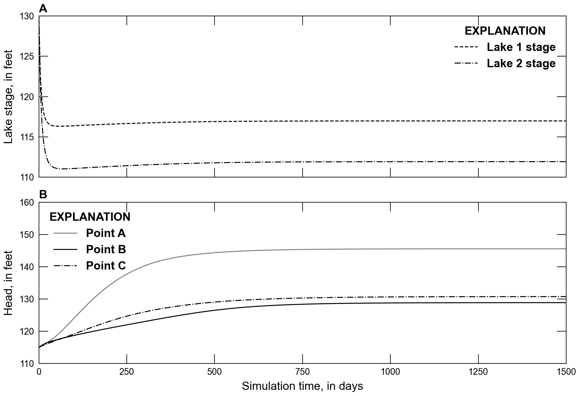
Figure 15.2 Lake stages and selected heads in the aquifer. A. Lake stages. The location of lake 1 and 2 are shown in Figure 15.1. B. Heads in the aquifer. The location of points A, B, and C are shown in Figure 15.1.
The stream system acts as a highly effective drain for the lake/aquifer system. The depth of flow in stream connecting lake 1 and 2 is about 2.1–2.3 \(ft\) and the depth of flow in stream discharging from lake 2 is generally is about 1.6–2 \(ft\). The volume of water leaking from the aquifer to the stream generally is about 2 to 7 percent of the downstream flow in each reach.
15.3. References Cited
Merritt, M. L., & Konikow, L. F. (2000). Documentation of a computer program to simulate lake-aquifer interaction using the MODFLOW ground-water flow model and the MOC3D solute-transport model. Retrieved from https://pubs.er.usgs.gov/publication/wri004167
15.4. Jupyter Notebook
The Jupyter notebook used to create the MODFLOW 6 input files for this example and post-process the results is: