11. Streamflow Routing Package Problem 1
This example is a modified version of the Streamflow Routing (SFR) Package described in (Prudic et al., 2004). The problem has been modified by converting all of the SFR reaches to use rectangular channels.
11.1. Conceptual Model
The example represents a hypothetical problem of stream-aquifer interaction for an alluvial basin in a semiarid region in which recharge to the aquifer is primarily leakage from streams that enter the basin from mountains on the northwest, northeast, and southeast (Figure 11.1).
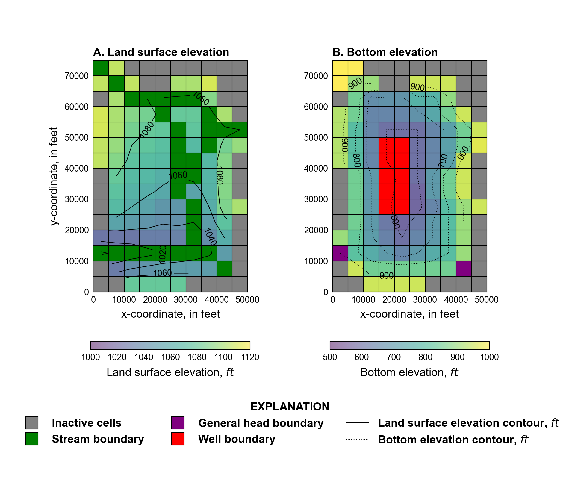
Figure 11.1 Land surface and aquifer bottom elevations. A. Land surface elevation. The location of inactive cells and cells with streamflow routing reaches are also shown. B. Aquifer bottom elevations. The location of cells with general-head and well boundaries are also shown.
The principal aquifer is unconsolidated deposits of mostly sand and gravel. The mountains consist of bedrock that is many times less permeable than the unconsolidated deposits. Upland areas adjacent to the basin contribute some recharge to the aquifer either as underflow through the perimeter bedrock or from intermittent channels that have small drainage areas. The southern stream is perennial across the valley. Groundwater flow trends in the same direction as the streams.
11.2. Example Description
Model parameters for the example are summarized in Table 11.1. The model consists of a grid of 10 columns, 15 rows, and 1 layer. The model domain is 50,000 \(ft\) and 80,000 \(ft\) in the x- and y-directions, respectively. The discretization is 5,000 \(ft\) in the row and column direction for all cells. The top of the model ranges from about 1,000 to 1,100 \(ft\) (Figure 11.1A) and the bottom of the model ranges from about 500 to 1,000 \(ft\) (Figure 11.1B).
Three stress periods are simulated. The first stress period is steady state and the remaining stress periods are transient. The stress periods are 0, 50, and 50 years in length and are broken up into 1, 50, and 50 time steps. A time step multiplier of 1, 1.1, and 1.1 are used in stress periods 1 through 3. respectively.
Parameter |
Value |
|---|---|
Number of periods |
3 |
Number of layers |
1 |
Number of rows |
15 |
Number of columns |
10 |
Column width (\(ft\)) |
5000.0 |
Row width (\(ft\)) |
5000.0 |
Starting head (\(ft\)) |
1050.0 |
Hydraulic conductivity near the stream (\(ft/s\)) |
0.002 |
Hydraulic conductivity in the basin (\(ft/s\)) |
0.0004 |
Specific storage (\(1/s)\) |
1e-6 |
Specific yield near the stream (unitless) |
0.2 |
Specific yield in the basin (unitless) |
0.1 |
Evapotranspiration rate (\(ft/s\)) |
9.5e-8 |
Evapotranspiration extinction depth (\(ft\)) |
15.0 |
The basin fill thickens toward the center of the valley and hydraulic conductivity of the basin fill is highest in the region of the stream channels. Hydraulic conductivity is 173 \(ft/day\) (\(2 \times 10^{-4}\) \(ft/s\)) in the vicinity of the stream channels and 35 \(ft/day\) (\(4 \times 10^{-4}\) \(ft/s\)) elsewhere in the alluvial basin. A constant specific storage value of \(1 \times 10^{-6}\) (\(1/day\)) was specified throughout the alluvial basin. Specific yield is 0.2 (unitless) in the vicinity of the stream channels and 0.1 (unitless) elsewhere in the alluvial basin.
An initial head of 1,050 \(ft\) is specified in all model layers. Any initial head exceeding the bottom of each cell could be specified since the model is steady-state.
Flow into the system is from infiltration from precipitation and was represented using the recharge (RCH) package. Recharge rates applied to each cell ranged \(2.5 \times 10^{-10}\) to \(2 \times 10^{-9}\) \(ft/s\), with lower rates in the vicinity of the stream channels and higher rates elsewhere in the alluvial basin. Flow out of the model is from groundwater evapotranspiration represented by evapotranspiration (EVT) package cells and discharging wells represented by well (WEL) package cells. Groundwater evapotranspiration occurs where depth to water is within 15 \(ft\) of land surface, has a maximum rate of 3 \(ft/yr\) at land surface, and is coincident with the valley lowland through which several streams flow. Wells are only active in the second stress period and were located in ten cells (rows 6 through 10 and columns 4 and 5) along the west side of the valley (Figure 11.1B). Each well extracted 10 \(ft^{3}/s\) of groundwater for a total withdrawal rate of 100 \(ft^{3}/s\) (about twice the steady-state ground-water inflow). Two general-head boundary cells were added in (row 13, column 1) and (row 14, column 8) with a specified head equal to 988 and 1,045 \(ft\), respectively, and a constant conductance of 0.038 \(ft^{2}/s\).
The streams in the model domain were represented using a total of 36 reaches. External inflows of 25, 10, and 100 \(ft^{3}/s\) were specified for reach 1, 16, and 28, respectively. Reach 1 is located in (row 1, column 1), reach 16 is in (row 5, column 10), and reach 28 is in (row 14, column 9). Streamflow discharges from the model at the downstream end of reach 36 in (row 13, column 1). Reach widths were specified to be 12, 0, 5, 12, 55, and 40 \(ft\) for reaches 1–9, 10–18, 19–22, 23–27, 28–30, and 31–36, respectively. The remaining streambed properties and stream dimensions used for each stream reach are the same as those used in (Prudic et al., 2004) (see Prudic et al., 2004Table 1). Constant stage reaches were used to define the ditch represented by reaches 10–15 and ranged from approximately 1,075.5–1061.6 \(ft\). A diversion from reach 4 to 10 was specified to represent managed inflows to the ditch. Ditch inflows were specified to be 10 \(ft^{3}/s\) except if the downstream flow in reach 4 is less than the specified diversion rate; in cases where the downstream flow in reach 4 is less than the specified diversion rate all of the downstream flow in reach 4 is diverted to the ditch and the inflow to reach
The model uses the Newton-Raphson Formulation. The simple complexity Iterative Model Solver option and preconditioned bi-conjugate gradient stabilized linear accelerator is also used.
11.3. Example Results
Simulated results for the initial steady-state stress period and at the end of the stress period with groundwater pumping (stress period 2) are shown in Figure 11.2. Reach stage and downstream discharge were also evaluated for reach 4, 14, 27, and 36.
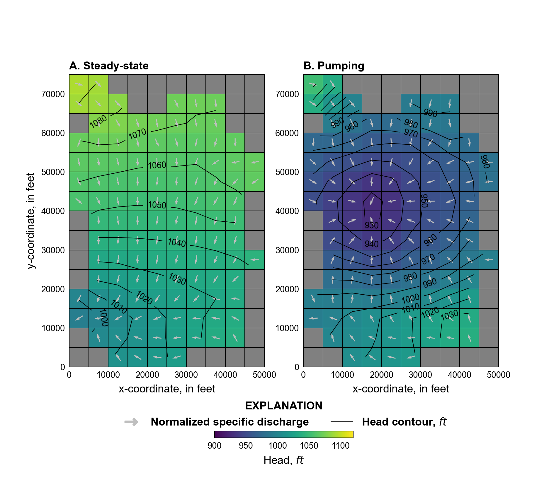
Figure 11.2 Simulated water levels and normalized specific discharge vectors under steady state and pumping conditions. A. steady-state results. B. results after 50 years of pumping.
Simulated stage and flow for reach 4 in (row 3, column 4) is shown in Figure 11.3A and B. Flow out decreased rapidly when pumping began, but the decrease slowed after only 3 years. The marked change in flow and stream depth was caused by a decline in ground-water levels relative to the head in the stream for all cells corresponding to all the upstream reaches. After 3 years, cells upstream of the reach 4 began to decline below the streambed causing the slope of the decline in flow to decrease. Flow in the stream no longer changed after about 9 years of pumping because the groundwater level in cells corresponding to the reaches upstream of reach 4 had declined below the streambed and the leakage rates had become constant. Once withdrawals ceased, flow began to increase in the last reach of segment 5 after about 21 yrs after pumping had ceased and after about 19 yrs in reach 4. The increase of flow in reach 4 during the recovery period was slower than the decrease in flow during the pumping period and largely was controlled by the gradual recovery of ground-water levels in areas distant from the pumping wells.
The last reach (reach 15) along the ditch (reaches 10–15) was used to illustrate how the option of specifying stream stage works when flow in a channel ceases and when flow commences again (Figure 11.3C and D). The stream stage and related depth is constant in reaches 10–15 as long as there is flow in the reach. Once flow in the reach ceases, the streambed elevation (depth = 0) is used for comparing head differences between the stream and groundwater. The slight lag between when flow out of the reach went to zero and when stream depth went to zero during the rapid decline was the result of all inflow into the reach leaking through the streambed. Inflow into the reach ceases during the following time step and consequently the entire reach became dry and stream depth became zero. The same lag occurred during the recovery period and was again caused by all inflow into the reach leaking through the streambed. Outflow from the last reach did not occur until inflow into the reach exceeded that which could leak through the streambed.
Flow in reach 27 (Figure 11.3E and F) is used to illustrate what happens when there is no inflow from upstream reaches, but the groundwater level in the corresponding model cell is higher than the elevation of the streambed. Flow and stream depth decreased rapidly in the pumping (second stress) period and depth became zero after only 2 years, even though there was still a small quantity of outflow from the reach. The reason for stream depth being zero with minor outflow is that the only source of water to the reach is from ground-water leakage. When this occurs, stream depth at the midpoint of the reach is set to zero and the stream head at the midpoint is equal to the streambed elevation.
In the steady-state stress period (stress period 1), reach 36 is generally gaining, but became losing during the pumping period (stress period 2) . Streamflow out of the reach and the depth decreased during the pumping period (Figure 11.3G and H) because inflow from upstream reaches declined and because leakage in the reach switched from flow out of the aquifer into the stream to flow from the stream into the aquifer. Although the water table declined in all cells corresponding to reaches 28–36, the water table did not decline below the streambed and consequently, streambed leakage did not become constant. Once pumping ceases, flow in the reach increases in a manner similar to how it decreased. The slight increase in flow after 70 years was due to an increase in flow from reaches upstream of reach 27. The response in reach 36 after pumping ceases in stress period 3 was much different than that for reach 4 and 27 (compare Figure 11.3H with Figure 11.3B) because groundwater levels did not decline below the bottom of the streambed beneath reaches 31–36 whereas they did beneath reaches 1–4.
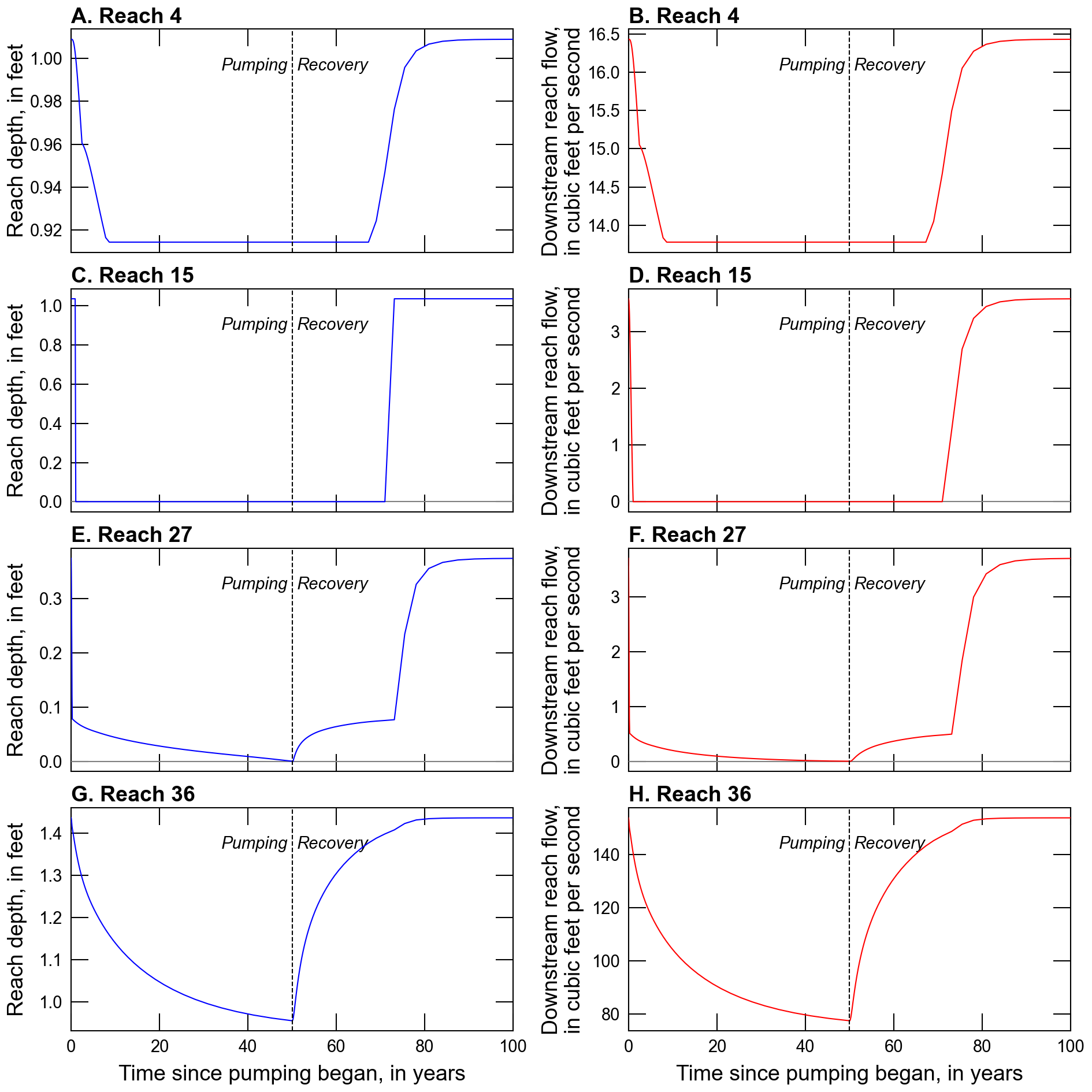
Figure 11.3 Simulated reach depth and downstream discharge at select reaches. A. Stage in reach 4. B. Downstream discharge in reach 4. C. Stage in reach 15. D. Downstream discharge in reach 15. E. Stage in reach 27. F. Downstream discharge in reach 27. G. Stage in reach 36. H. Downstream discharge in reach 36.
11.4. References Cited
Prudic, D. E., Konikow, L. F., & Banta, E. R. (2004). A new streamflow-routing (SFR1) package to simulate stream-aquifer interaction with MODFLOW-2000. Retrieved from https://pubs.er.usgs.gov/publication/ofr20041042
11.5. Jupyter Notebook
The Jupyter notebook used to create the MODFLOW 6 input files for this example and post-process the results is: