26. CSUB Package Problem 3

A one-dimensional MODFLOW 6 model was developed by (Sneed, 2008) to simulate aquitard drainage, compaction and, land subsidence at the Holly site, located at the Edwards Air Force base, in response to effective stress changes caused by groundwater pumpage in the Antelope Valley in southern California (Figure 26.1). Land subsidence resulting from groundwater level declines, has long been recognized as a problem in Antelope Valley, California. The original one-dimension compaction model was calibrated to extensometer data from the USGS Holly site (station name 008N010W01Q005S) for the period from 1990 to 2006, and used a head based-formulation to represent compaction. The model of (Sneed, 2008) has been modified to use the effective stress formulation available in the CSUB package for MODFLOW 6.

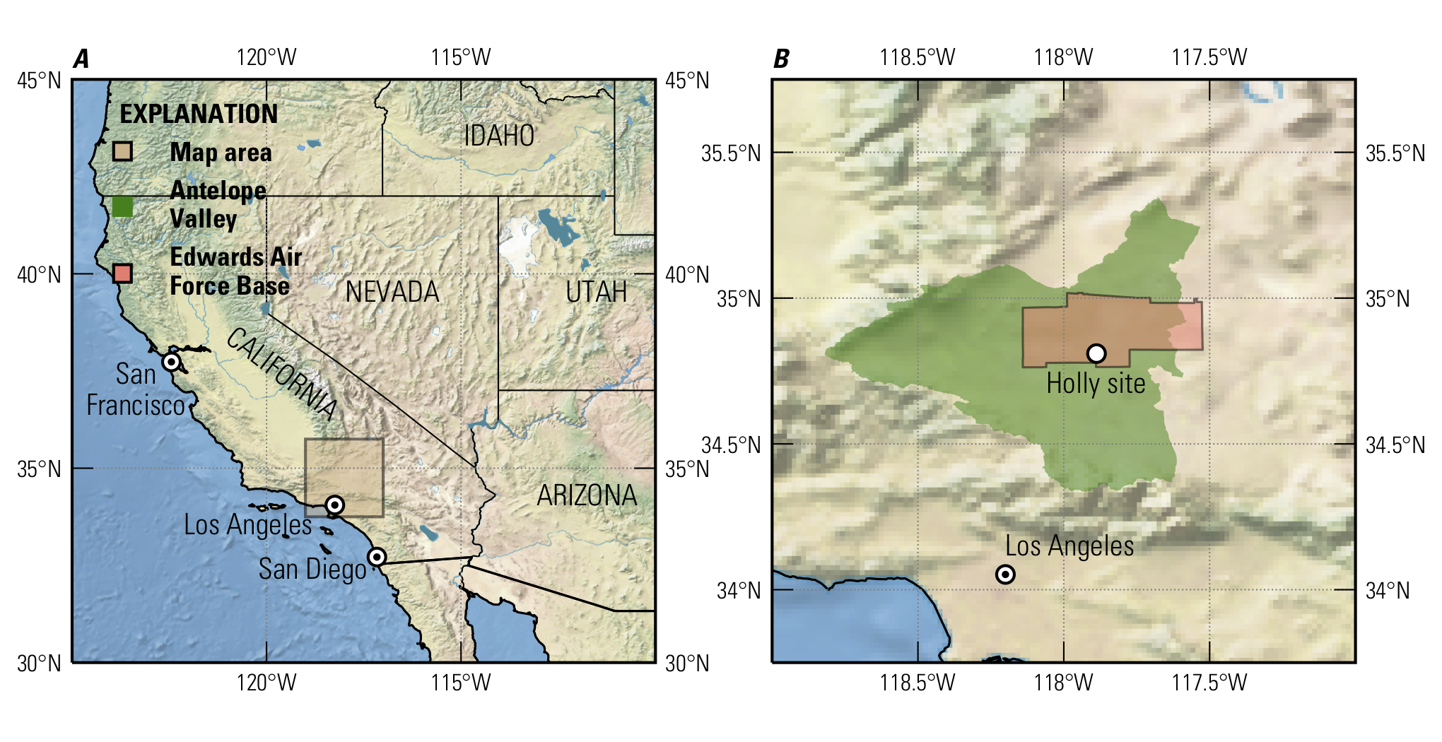
Figure 26.1 Maps showing the location of the study area for the one-dimensional compaction problem in southern California. A, location of the study area in southern California and B, location of the Holly site and Edwards Air Force Base in the Antelope Valley. Cross-blended hypsometric tints with relief, water, drains and ocean bottom background image from Natural Earth and is available at https://www.naturalearthdata.com/downloads/50m-raster-data/50m-cross-blend-hypso/, accessed on July 9, 2019

26.1. Site Description

The subsurface geology at the Holly site comprises Quaternary alluvial and lacustrine deposits from land surface to about 260 meters below land surface, consolidated late Tertiary and early Quaternary sedimentary continental deposits from about 260 to 330 meters below land surface, and decomposed basement complex. Lithologic and geophysical logs of the Holly site indicate the presence of relatively thin interbedded aquitards, ranging from 0.3 to 5 meters thick, and two thicker aquitards 20 meters (37–57 meters below land surface) and 19 meters (92–111 meters below land surface) thick. The upper aquitard is interpreted as a regionally extensive, confining unit. The groundwater system at the Holly site is comprises two aquifer systems–an unconfined system and a confined system, which are separated by lacustrine blue-clay deposits that constitute the confining unit. The upper aquifer is unconfined, about 37 meters thick and the water table is about 20 meters below land surface. The confined-aquifer system at the site extends about 275 meters below the confining unit, where it is underlain by weathered bedrock. The middle aquifer is the source of most of the groundwater pumped from the well field closest to the Holly site. Additional information on the hydrogeology of the Holly site and the Antelope Valley can be found in (Sneed & Galloway, 2000) and (Sneed, 2008).

Compaction at the Holly site for the period from 1990 through 2006 was measured using a counterweighted pipe extensometer designed to measure compaction in the interval from 4.6 to about 260 meters below land surface. The principal mode of compaction at the Holly site is a seasonally dependent step response. Larger rates of compaction are associated with summer water-level drawdowns and despite groundwater level recoveries of more than 3 meters during the winter, compaction continues, at a reduced rate. The absence of aquifer-system expansion during seasonal water-level recovery is consistent with the delayed drainage and resultant delayed, or residual, compaction of thick aquitards.

26.2. Example Description

The model grid for this problem consists of 14 layers, 1 row, and 1 column (Figure 26.2). The model layers are based on the model of (Sneed, 2008), with the exception of the top of model layer 1 which was modified from the original value of -27.74 meters to 0 meters to allow the model to account for unsaturated conditions above the water table when calculating geostatic and effective-stresses. Model layer thicknesses are summarized in Table 26.1. DELR and DELC are equal to 1 meter. The model consists of 353 stress periods covering the period from May 8, 1908 to September 4, 2006. The duration of model stress periods and time steps for the period from May 8, 1908 to May 9, 1990 (“early time”) were annual and monthly–365.25 and 30.4375 days, respectively, and were 22 and 1 days, respectively, for the period from May 9, 1990 to September 4, 2006 (“late time”). The nearly century duration of the simulations allows for comparisons of aquifer-system compaction owing to sustained groundwater pumpage and water-level declines through the period of groundwater development and seasonal groundwater level cycling since 1990.

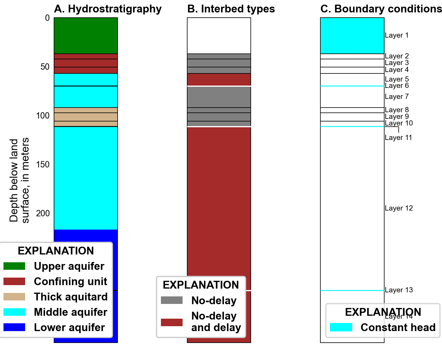
Figure 26.2 Diagram showing the model domain and setup for the one-dimensional compaction problem. A, hydrostratigraphy, B, interbed types used in aquifer and confining units, and C, location of constant-head boundary conditions

Table 26.1 Aquifer properties for example ex-gwf-csub-p03.

Layer	Thickness	Hydraulic conductivity	Initial head
1	36.88	9.14e-3	0.00
2	5.49	3.66e-6	1.57
3	8.23	3.66e-6	3.38
4	6.40	3.66e-6	5.56
5	12.80	9.14e-3	6.77
6	0.30	9.14e-3	6.77
7	21.95	9.14e-3	6.77
8	5.18	4.57e-6	6.77
9	8.53	4.57e-6	6.77
10	5.49	4.57e-6	6.77
11	0.30	9.14e-3	6.77
12	167.34	9.14e-3	6.77
13	0.30	9.14e-3	5.55
14	53.34	9.14e-3	5.55

Hydraulic properties used in the model are shown in Table 26.1. (Sneed, 2008) specified different horizontal and vertical hydraulic conductivity values for each layer; however, vertical hydraulic conductivity values from (Sneed, 2008) were assigned as the horizontal hydraulic conductivity values in each layer since there is no horizontal flow in this one-dimensional problem. The specific yield and specific storage in the STO package were defined to be 0 for all layers. All model layers are defined to be non-convertible for hydraulic conductivity and storage properties. Default NPF and STO package settings were used. Initial heads in the model range from 0. to 6.77 meters (Table 26.1).

The effective stress formulation of the CSUB package was used to simulate compaction of aquifer materials. Fine-grained materials defined as delay interbeds were were discretized using 39 cells and assigned a uniform vertical hydraulic conductivity of \(4.57 \times 10^{-6}\) meters per day. A specific gravity of 1.7 and 2.0 was defined for moist and saturated sediments, respectively. Water compressibility was simulated using a specific gravity of water of 9,806.65 Newtons per cubic meters and water compressibility of \(4.6512 \times 10^{-10}\) per Pascal. The thickness of compressible materials and total porosity were updated during the simulation in response compaction.

Interbedded aquitards ranged from 0.3 to 5.5 meters in thickness. The Holly model simulates interbedded aquitards less than 1.5 meters thick using no-delay interbeds (ultimate compaction occurs within a model time step), and simulates interbedded aquitards 1.5 meters thick or greater using delay-interbeds (ultimate compaction does not occur within a model time step). A total of 18 interbedded aquitards ranging from approximately 0.3 to 1.2 meters thick, with a total aggregate thickness of approximately 12 meters, were modeled as no-delay interbeds and 10 interbedded aquitards ranging from approximately 1.5 to 5.5 meters thick, with a total aggregate thickness of approximately 27 meters, were modeled as delay interbeds (Table 26.2). The confining unit (approximately 20 meters thick) and the thick aquitard (approximately 19 meters thick), were modeled as no-delay interbeds (Table 26.2). Simulation of delayed drainage and residual compaction in each of these units was simulated implicitly using 3 model layers as recommended in (Hoffmann et al., 2003). Compaction was not simulated for the upper aquifer because the upper aquifer is relatively coarse grained and heads are changing very slowly and are hydraulically isolated from seasonal groundwater fluctuations in the production zones of the aquifer system. A constant porosity of 0.30 was used for the coarse- and fine-grained materials in the model.

Table 26.2 Interbed properties for example ex-gwf-csub-p03.

Interbed	Layer	Thickness	Initial stress
1	2	5.49	47.27
2	3	8.23	55.93
3	4	6.40	62.76
4	5	2.74	75.90
5	7	0.61	98.15
6	8	5.18	103.33
7	9	8.53	111.86
8	10	5.49	117.35
9	12	7.62	285.60
10	14	0.91	339.25
11	5	5.27	75.90
12	12	5.06	285.60
13	14	7.82	339.25

Initial preconsolidation stresses were calculated from initial preconsolidation heads developed by (Sneed, 2008) and effective stresses calculated using initial heads (Table 26.1). Initial preconsolidation stresses for no-delay and delay interbeds are summarized in Table 26.2, respectively. (Sneed, 2008) estimated initial preconsolidation heads from the time series for paired bench marks near the Holly site and middle aquifer water levels (Figure 26.3). Delay beds in the middle aquifer (model layers 5 and 12) and the lower aquifer (model layer 12) were specified to be 6.77 and 5.55 meters above land surface, respectively, which are the same as initial heads in these layers.

Boundary conditions in the one-dimensional compaction model of the Holly site consist of constant (time-variant) heads for those parts of the coarse-grained aquifer that represent measured (or estimated) hydraulic head (Figure 26.2C). The upper, middle, and lower aquifers at the Holly site are represented in the model by specifying heads in each aquifer using data from (Sneed, 2008) and are shown in Figure 26.3. The upper model boundary is a time-variant, constant-head boundary that represents measured or estimated heads in the upper aquifer (model layer 1) at the Holly site and is about 28 meters below land surface (Figure 26.2C). Three boundaries within the model domain consist of time-variant, specified heads that represent measured or estimated heads in the middle (model layers 6 and 11) and lower aquifers (model layer 13) at the Holly site (Figure 26.2C). Time-varying heads for constant-head cells were defined using a time series file. Although compaction is not thought to be important in the upper aquifer it should be noted that compaction and related release/storage of water are not simulated in cells with constant-head boundaries.

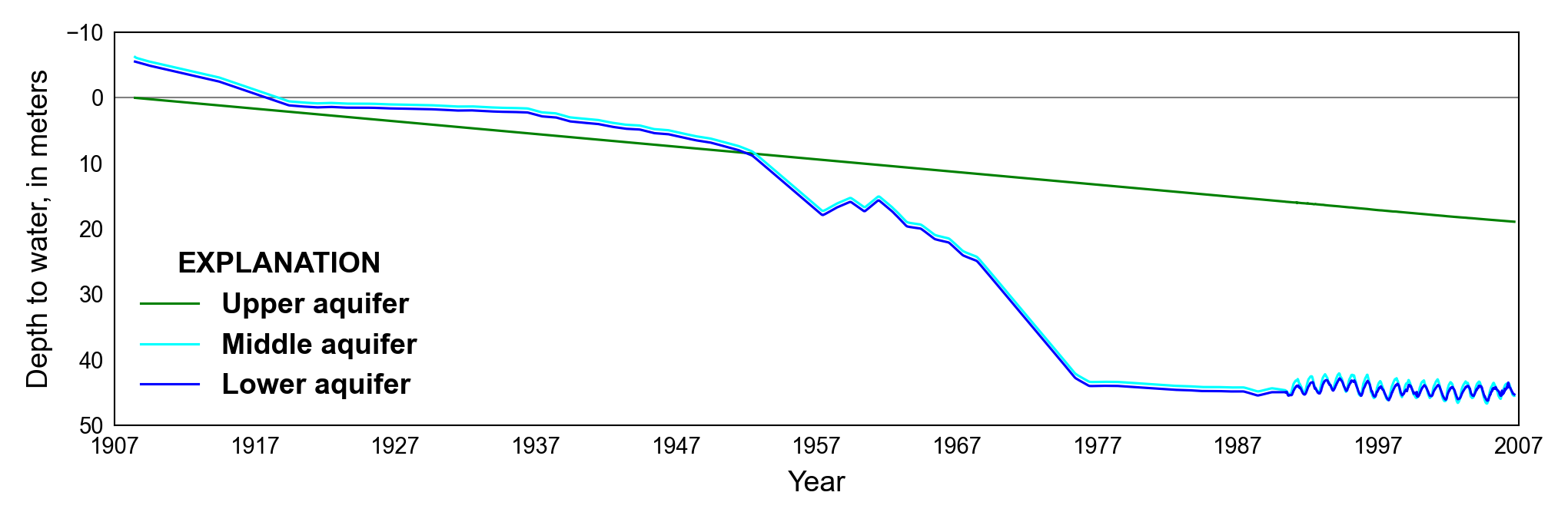
Figure 26.3 Graph showing depth to water values used in the one-dimensional compaction problem for the upper, middle, and lower aquifers at the Holly site, Edwards Air Force Base, Antelope Valley, California. Modified from (Sneed, 2008)

The compaction at the end of the simulation for the confining unit (0.28 meters), the thick aquitard (0.66 meters), no-delay interbeds contained in aquifer units (0.06 meters), delay interbeds contained in aquifer units (0.35 meters), and coarse grained materials (0.06 meters) from a modified MODFLOW 6 version of the model of (Sneed, 2008) were used to calibrate initial specific storage values used in the model. The specific storage values used by (Sneed, 2008) were uniformly scaled by a factor of \(9.9408 \times 10^{-1}\) to better match the observed compaction at the Holly site for the period from October 1, 1992 to May 9, 2006. The total compaction at the end of the simulation period (1.42 meters) and the total compaction from October 1, 1992 to May 9, 2006 (0.19 meters) were also used to calibrate initial specific storage values used in the model.

PEST++ (Welter et al., 2015) was used to calibrate 1) the elastic specific storage value for coarse grained materials in model layers 5, 7, 12, and 14; 2) inelastic and elastic specific storage values for the confining unit (model layers 2–4); 3) inelastic and elastic specific storage values for the thick aquitard (model layers 8–10); and 4) inelastic and elastic specific storage value were calibrated for no-delay and delay interbeds contained in aquifer units (model layers 5, 6, 12, and 14). Compaction values simulated using the head-based formulation for the confinining unit, the thick aquitard, no-delay interbeds contained in aquifer units, delay interbeds contained in aquifer units, and coarse grained materials were given a weight of 1; total compaction and the total compaction from October 1, 1992 to May 9, 2006 were given an increased weight of 5 to favor fitting the total compaction and observed change in total compaction over material based compaction values.

26.3. Example Results

Comparison of head- and effective stress-based compaction results are shown in Figure 26.4. The compaction at the end of the simulation in the model using head- and effective stress-based formulation were essentially identical and mean errors calculated for the entire simulation ranged from -0.0045 meters (confining unit compaction) to 0.0042 meters (compaction in delay interbeds contained in aquifer units), with the largest differences occurring between approximately 1947 and 1977.

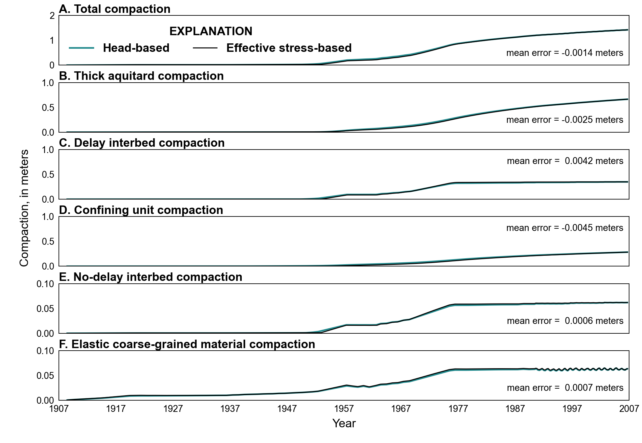
Figure 26.4 Graphs showing simulated compaction in different material types using head- and effective stress based formulations for the one-dimensional compaction problem. A, Total compaction, B, compaction in interbeds in the thick aquitard, C, compaction in delay interbeds contained in aquifers, D, compaction in interbeds in the confining unit, E, compaction in no-delay interbeds contained in aquifers, and F, compaction in coarse-grained materials

The thickness of compressible materials and calibrated specific storage values for coarse-grained materials, fine-grained materials represented as no-delay interbeds, and fine-grained materials represented as delay interbeds are summarized in tables Table 26.3 and Table 26.4, respectively. Calibrated specific storage values are larger than values used with the head-based formulation. Percent differences relative to values used by (Sneed, 2008) were 27.0% for the elastic specific storage values of coarse-grained materials, averaged 79.2 and 210.2% for the inelastic and elastic specific storage values of no-delay interbeds, and averaged 20.6 and 52.2% for the inelastic and elastic specific storage values of delay interbeds. Larger specific storage values are expected for the effective stress-based formulation since effective-stress values increase during the simulation, as a result of groundwater pumpage induced water-level declines, and result in reduced specific storage values and compaction with time relative to the head-based formulation model using the uniformly scaled specific storage values from (Sneed, 2008).

Table 26.3 Aquifer storage properties for example ex-gwf-csub-p03.

Layer	Specific Storage
5	6.88e-6
7	6.88e-6
12	6.88e-6
14	6.88e-6

Table 26.4 Interbed storage properties for example ex-gwf-csub-p03.

Interbed	Layer	Inelastic Specific Storage	Elastic Specific Storage
1	2	1.35e-3	8.57e-6
2	3	1.35e-3	8.57e-6
3	4	1.35e-3	8.57e-6
4	5	2.69e-4	1.26e-5
5	7	2.71e-4	1.15e-5
6	8	1.92e-3	3.42e-5
7	9	1.92e-3	3.42e-5
8	10	1.92e-3	3.42e-5
9	12	1.46e-4	6.40e-6
10	14	2.17e-4	9.24e-6
11	5	2.27e-4	1.03e-5
12	12	4.87e-4	7.59e-6
13	14	1.02e-3	6.86e-6

The simulations for the period 1908–2006 provide information about how the aquifer-system components, aquifers and aquitards, contributed to overall compaction because of the continual lowering of water levels throughout the 1900s and because of seasonal water-level cycling since 1990. Simulated compaction totaled 1.42 meters for the period 1908–2006. Of the total simulated compaction, the confining unit (thickness = 20.12 meters) accounted for 20.0% of the total; the thick aquitard (thickness = 19.20 meters) accounted for 46.7% of the total; delay interbeds in aquifers (aggregate thickness = 18.14 meters) accounted for 24.6%; coarse-grained materials (aggregate thickness = 225.39 meters) accounted for 4.5% of the total; and no-delay interbeds in aquifers (aggregate thickness = 11.89 meters) accounted for 4.4% of the total (Figure 26.5A). During 1990–2006, a total of 0.23 meters of compaction was simulated; the confining unit accounted for 31.2% of the total; the thick aquitard accounted for 66.3% of the total; delay interbeds in aquifers accounted for 1.7%; coarse-grained materials accounted for -0.1% (representing expansion of coarse grained materials); and no-delay interbeds in aquifers accounted for 0.9% of the total. For these relatively quickly equilibrating thin aquitards, the fairly stable stresses since the mid-1970s and cyclic stresses during the late time were often in the elastic range of stress. In fact, beginning in about 1976, the delay and no-delay interbeds in aquifers had significantly reduced compaction rates, contributing only 0.01 meters (2.4%) and 0.004 meters (0.1%) of compaction, respectively, during the last 30 years of the simulation. These thin aquitards deformed mostly elastically during the late time (Figure 26.5).

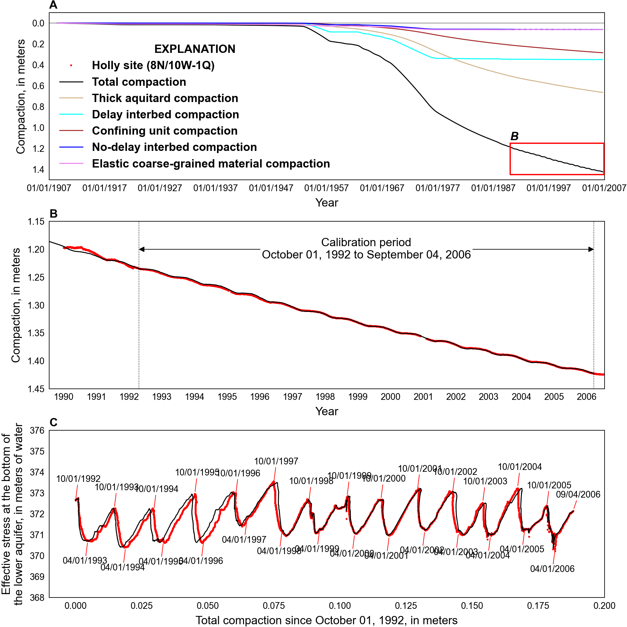
Figure 26.5 Graphs showing history matches for simulated and measured aquifer-system compaction in the one-dimensional compaction problem. A, compaction in the different material types for the full simulation period (for 1908–2006 ), B, comparison of simulated and observed compaction at the Holly site for the period from 1990 to 2007, and C, simulated and observed stress/displacement for the period from October 1, 1992 to September 4, 2006. Elastic and inelastic specific storage values were calibrated using observed Holly site compaction data for the period from October 1, 1992 to September 4, 2006 and simulated compaction from the model based on (Sneed, 2008), which used a head-based formulation to simulate compaction

The simulated stress/displacement trajectory also compares well in magnitude and timing with the measured stress/displacement trajectory between October 1, 1992 and September 4, 2006 (Figure 26.5C). The effective stress at the base of the lower aquifer was estimated using water-level data for the upper and lower aquifers (Figure 26.3). The estimated stress/displacement trajectory fit is poorest from 1993 to 1996 when seasonal compaction changes lag behind observed changes. After April 1997, simulated compaction is generally consistent with observed compaction.

Vertical distributions of hydraulic head in the aquitards can be used as a direct measure of residual compaction (Riley, 1969, 1998). A linear profile showing deviations in the simulated 1908 to 2006 head distributions for the two thick clay sequences–the confining unit and the thick aquitard–indicate large residual excess pore pressures exist at the end of the simulation (Figure 26.6). Residual excess pore pressures in these thick aquitards began accumulating in about 1950, when water levels in the aquifers began declining at rate faster (Figure 26.3) than these aquitards could dissipate excess pore pressures. The simulations indicate that about 98% of the compaction during late time is residual compaction occurring in these two thick clay sequences (Figure 26.5A).

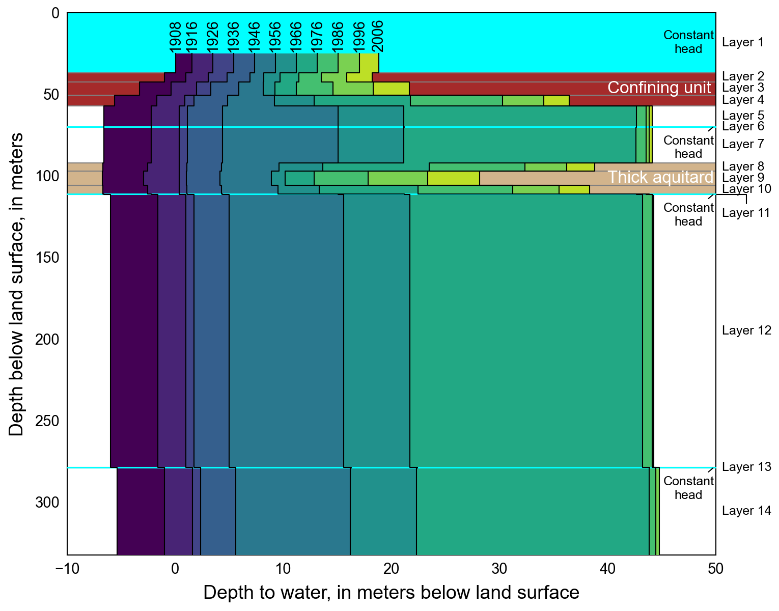
Figure 26.6 Graph showing simulated vertical head profiles and approximately decadal head changes in the one-dimensional compaction problem. Vertical head profiles are shown for 1908, 1916, 1926, 1936, 1946, 1956, 1966, 1976, 1986, 1996, and 2006. The colored area between plotted years represents the simulated head change over approximately decadal period of time between simulated vertical head profiles. The vertical location of model layer tops and bottom and layers with constant-head boundaries are also shown.

26.4. References Cited

Hoffmann, J., Leake, S. A., Galloway, D. L., & Wilson, A. M. (2003). MODFLOW-2000 Ground-Water Model—User Guide to the Subsidence and Aquifer-System Compaction (SUB) Package. Retrieved from https://pubs.usgs.gov/of/2003/ofr03-233/

Riley, F. S. (1969). Analysis of borehole extensometer data from Central California. International Association of Scientific Hydrology Publication 89, 2, 423–431.

Riley, F. S. (1998). Mechanics of aquifer systems—The scientific legacy of Joseph F. Poland. In Land subsidence case studies and current research: Proceedings of the Dr. Joseph F. Poland Symposium on Land Subsidence: Belmont, Calif., Star Publishing Co., Association of Engineering Geologists Special Publication (Vol. 8, pp. 13–27).

Sneed, M. (2008). Aquifer-system compaction and land subsidence: data and simulations, the Holly site, Edwards Air Force Base, California.

Sneed, M., & Galloway, D. L. (2000). Aquifer-system compaction and land subsidence: measurements, analyses, and simulations: the Holly Site, Edwards Air Force base, Antelope Valley, California. Retrieved from https://pubs.er.usgs.gov/publication/wri20004015

Welter, D. E., White, J. T., Hunt, R. J., & Doherty, J. E. (2015). Approaches in highly parameterized inversion–PEST++ Version 3, a Parameter ESTimation and uncertainty analysis software suite optimized for large environmental models. Retrieved from https://doi.org/10.3133/tm7C12

26.5. Jupyter Notebook

The Jupyter notebook used to create the MODFLOW 6 input files for this example and post-process the results is:

• ex-gwf-csub-p03