36. MOC3D Problem 2 with Triangular Grid
This problem corresponds to the second problem presented in the MOC3D report (Konikow et al., 1996), which involves the transport of a dissolved constituent in a steady, three-dimensional flow field. An analytical solution for this problem is given by (Wexler, 1992). As for the previous example, this example is simulated with the GWT Model in MODFLOW 6, which receives flow information from a separate simulation with the GWF Model in MODFLOW 6. In this example, however, a triangular grid is used for the flow and transport simulation. Results from the GWT Model are compared with the results from the (Wexler, 1992) analytical solution.
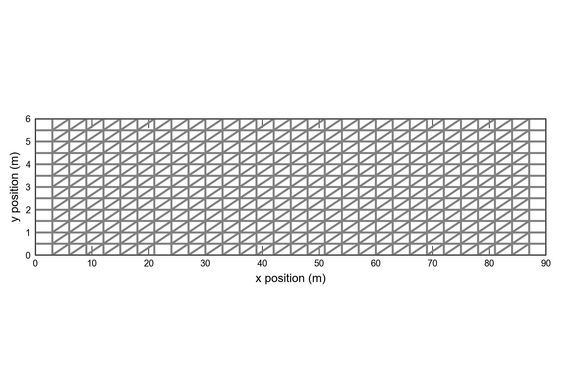
Figure 36.1 Triangular model grid used for the MODFLOW 6 simulation. Model grid is shown using an aspect ratio of 4.
36.1. Example description
(Wexler, 1992) presents an analytical solution for three dimensional solute transport from a point source in a one-dimensional flow field. As described by (Konikow et al., 1996), only one quadrant of the three-dimensional domain is represented by the numerical model. Thus, the solute mass flux specified for the model is one quarter of the solute mass flux used in the analytical solution.
The parameters used for this problem are listed in Table 36.1. The model grid for this problem consists of 40 layers, 695 cells per layer, and 403 vertices in a layer. The top for layer 1 is set to zero, and flat bottoms are assigned to all layers based on a uniform layer thickness of 0.05 \(m\). The remaining parameters are set similarly to the previous simulation with a regular grid, except for in this simulation, the XT3D method is used for flow and dispersive transport.
Parameter |
Value |
|---|---|
Number of periods |
1 |
Number of layers |
40 |
Number of rows |
12 |
Number of columns |
30 |
Column width (\(m\)) |
3 |
Row width (\(m\)) |
0.5 |
Layer thickness (\(m\)) |
0.05 |
Top of the model (\(m\)) |
0.0 |
Model bottom elevation (\(m\)) |
–2.0 |
Velocity in x-direction (\(m d^{-1}\)) |
0.1 |
Hydraulic conductivity (\(m d^{-1}\)) |
0.0125 |
Porosity of mobile domain (unitless) |
0.25 |
Longitudinal dispersivity (\(m\)) |
0.6 |
Transverse horizontal dispersivity (\(m\)) |
0.03 |
Transverse vertical dispersivity (\(m\)) |
0.006 |
Simulation time (\(d\)) |
400.0 |
Solute mass flux (\(g d^{-1}\)) |
2.5 |
Source location (layer, row, column) |
(1, 12, 8) |
36.2. Example Results
A comparison of the MODFLOW 6 results with the analytical solution of (Wexler, 1992) is shown for layer 1 in Figure 36.2.
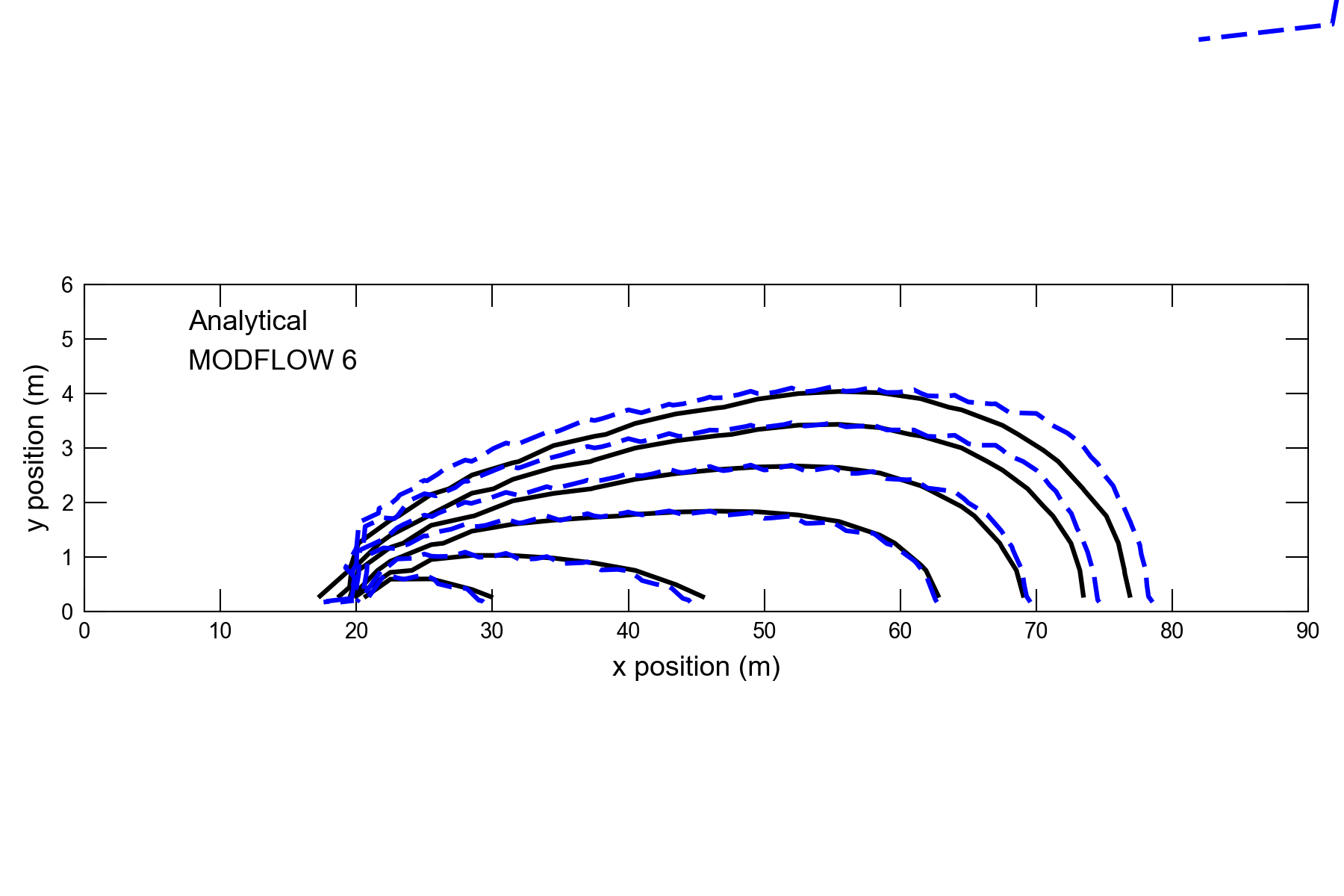
Figure 36.2 Concentrations simulated by the MODFLOW 6 GWT Model and calculated by the analytical solution for three-dimensional flow with transport. Results are for the end of the simulation (time=400 \(d\)) and for layer 1. Black lines represent solute concentration contours from the analytical solution (Wexler, 1992); blue lines represent solute concentration contours simulated by MODFLOW 6. An aspect ratio of 4.0 is specified to enhance the comparison.
36.3. References Cited
Konikow, L. F., Goode, D. J., & Hornberger, G. Z. (1996). A three-dimensional method-of-characteristics solute-transport model (MOC3D). Retrieved from https://pubs.er.usgs.gov/publication/wri964267
Wexler, E. J. (1992). Analytical solutions for one-, two-, and three-dimensional solute transport in ground-water systems with uniform flow.
36.4. Jupyter Notebook
The Jupyter notebook used to create the MODFLOW 6 input files for this example and post-process the results is: