24. Vilhelmsen LGR
This example reproduces several models described by (Vilhelmsen et al., 2012), which simulate groundwater flow in a buried valley aquifer at different grid resolution. The domain is simulated using a globally refined (GR) grid, a globally coarsened (GC) grid, and a coarse outer grid with a locally refined inset grid (LGR).
24.1. Example Description
Groundwater flow is simulated using three different simulations corresponding to three different grid configurations: GR, GC, and LGR (tab. Table 24.2). The GR grid consists of 25 layers, 183 rows and 147 columns. The grid spacing along rows is 35 \(m\) and the grid spacing along columns is 25 \(m\). The top of the model is variable, based on topography in the area (Figure 24.1). Layer bottoms are flat. The bottom for layer 1 is set to 30 \(m\). Bottom elevations for layers 2 through 25 are calculated using a uniform layer thickness of 5 \(m\). A cross section for the GR grid is shown in Figure 24.2.
The GC grid fits evenly into the GF grid, and has 1/3 the number of cells in the row and column directions. Instead of 25 layers, the GC grid has only 9 layers. Layer 1 corresponds to layer 1 in the GF model; however, each underlying layer in the GC grid corresponds to three layers in the GF model. The GC grid is shown in map view in Figure 24.3 and as a cross section in Figure 24.4.
The LGR grid is a combination of the GF and GC grids (Figure 24.5). The course outer parent grid is comprised of the GC grid, whereas the inset child grid consists of the GF grid. The LGR simulation consists of two separate model input files, one for the parent model and one for the child model. The two models are connected in MODFLOW 6 using the GWF-GWF Exchange, which is used to connect cells from the parent model to cells in the child model.
There are three different hydrogeologic units. The upper layer represents overburden material. The buried valley is filled with valley sediments, and the bottom material consists of the deposits into which the valley is incised. These three units are assigned a single value for hydraulic conductivity.
Recharge is uniformly applied to the water table at a rate of 1.1098e-9 \(m/s\). A river is represented in model layer 1 using the River (RIV) Package. The models are run as steady state using a single time step with a duration of 1 second.
Parameter |
Value |
|---|---|
Number of periods |
1 |
Number of layers in refined model |
25 |
Number of rows in refined model |
183 |
Number of columns in refined model |
147 |
Number of layers in coarsened model |
9 |
Number of rows in coarsened model |
61 |
Number of columns in coarsened model |
49 |
Column width (\(m\)) in refined model |
35.0 |
Row width (\(m\)) in refined model |
25.0 |
Layer thickness (\(m\)) in refined model |
5.0 |
Column width (\(m\)) in coarsened model |
105.0 |
Row width (\(m\)) in coarsened model |
75.0 |
Layer thickness (\(m\)) in coarsened model |
15.0 |
Top of the model (\(m\)) |
variable |
Layer bottom elevations (\(m\)) |
30 to –90 |
Cell conversion type |
0 |
Recharge rate (\(m/s\)) |
1.1098e-09 |
Horizontal hydraulic conductivity (\(m/s\)) |
5.e-07, 1.e-06, 5.e-05 |
Scenario |
Scenario Name |
Parameter |
Value |
|---|---|---|---|
1 |
ex-gwf-lgrv-gr |
configuration |
Refined |
2 |
ex-gwf-lgrv-gc |
configuration |
Coarse |
3 |
ex-gwf-lgrv-lgr |
configuration |
LGR |
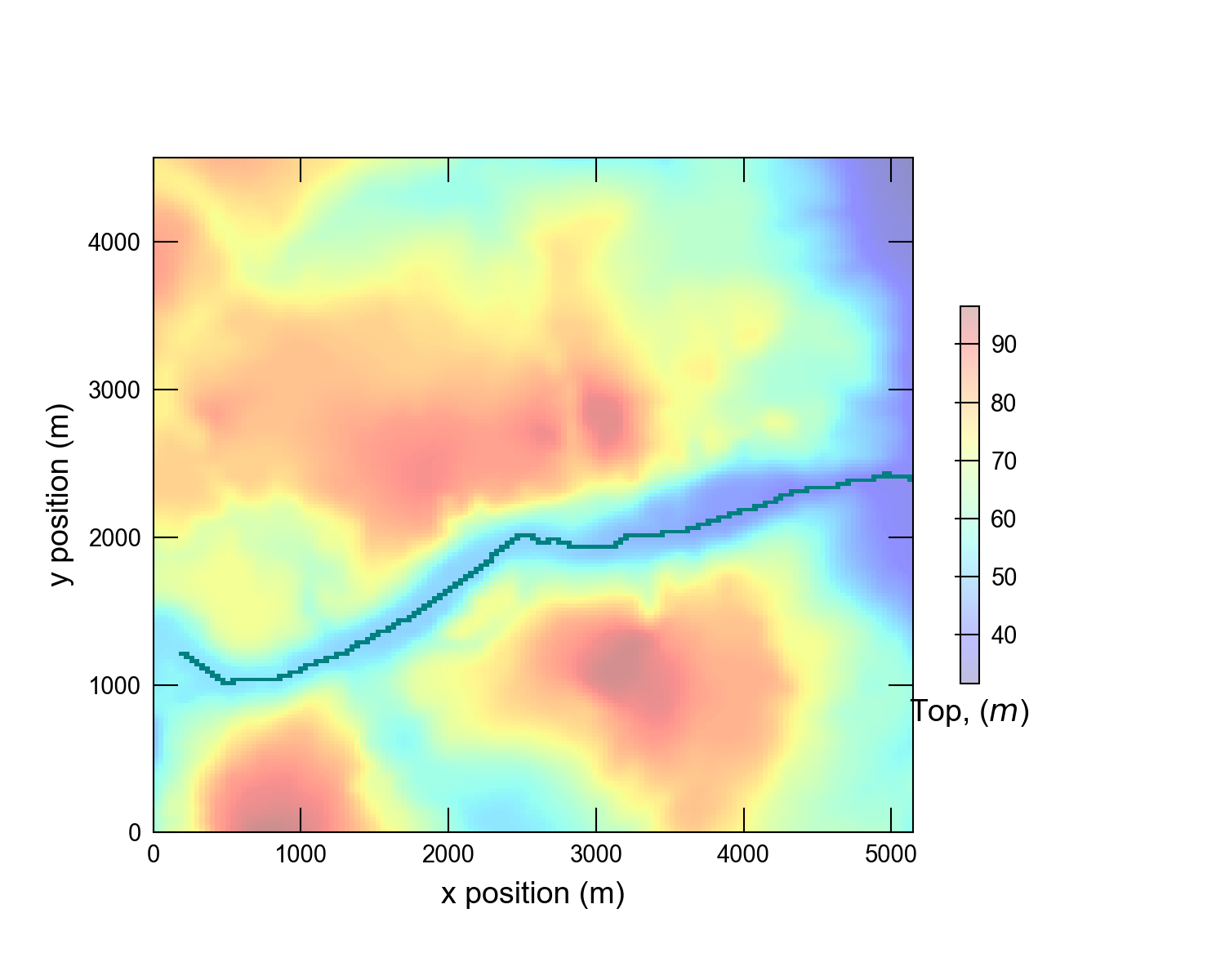
Figure 24.1 Globally refined model grid showing top elevation and river cells. Area of interest is shown as a dashed line.
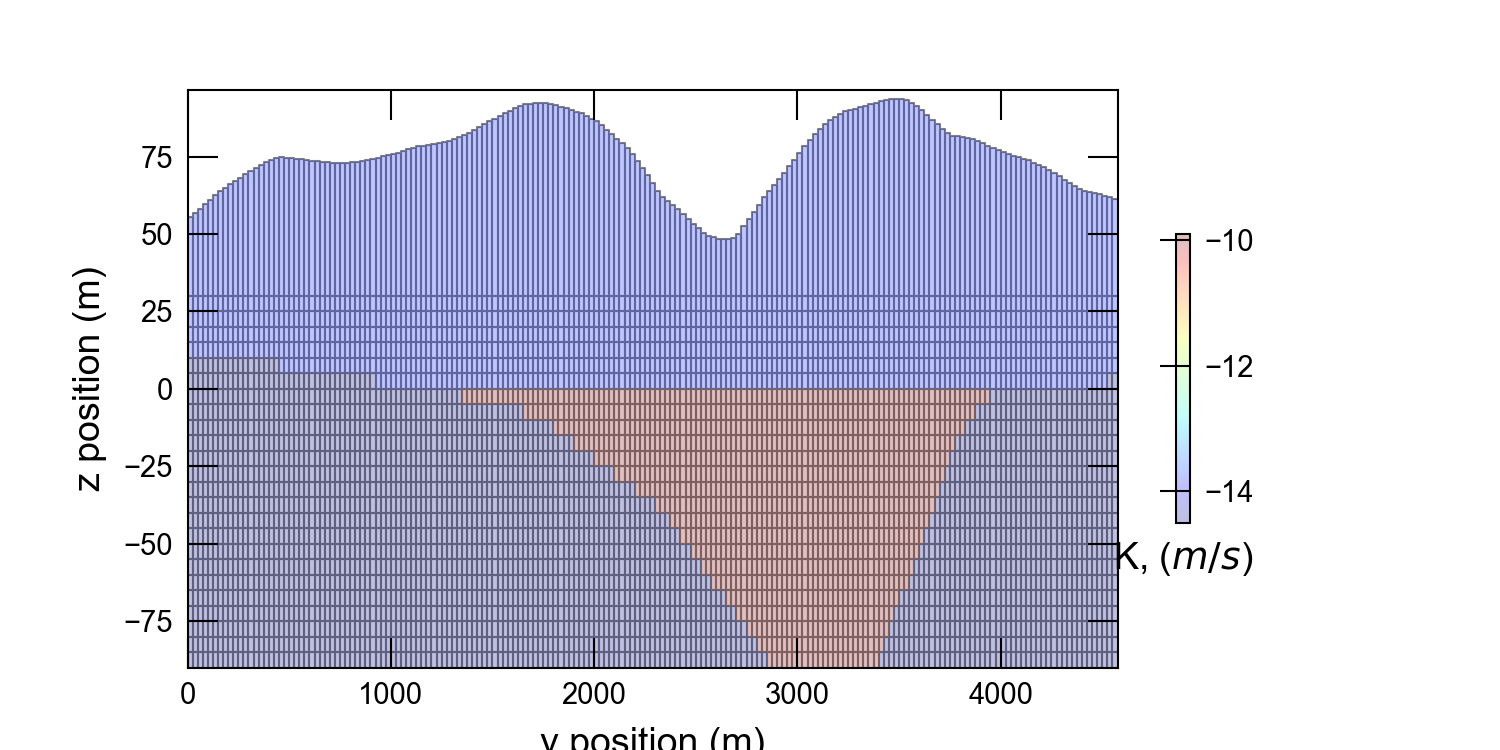
Figure 24.2 Cross section for y = 3000 \(m\) showing globally refined model grid. Color flood of hydraulic conductivity shows overburden material, valley fill, and deposits into which the valley is incised.
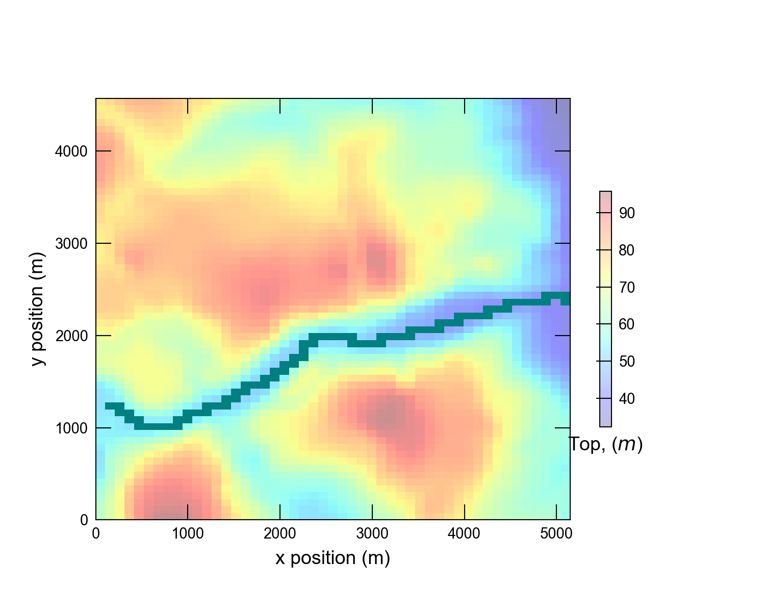
Figure 24.3 Globally coarsened model grid showing top elevation and river cells. Area of interest is shown as a dashed line.
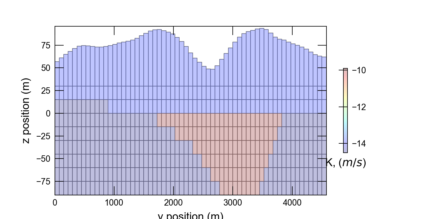
Figure 24.4 Cross section for y = 3000 \(m\) showing globally coarsened model grid. Color flood of hydraulic conductivity shows overburden material, valley fill, and deposits into which the valley is incised.
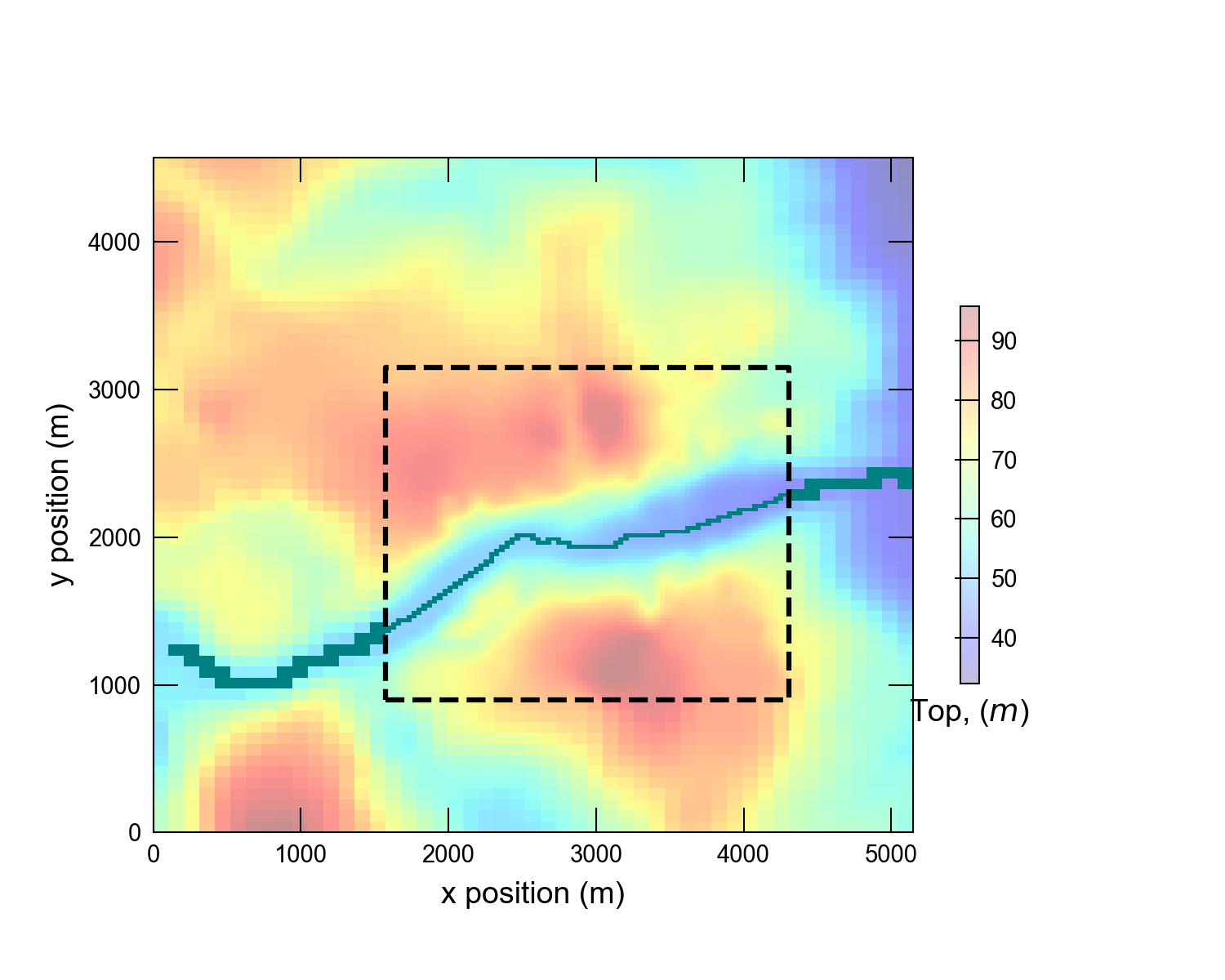
Figure 24.5 Local grid refinement model showing the outer coarse grid and the inner refined model grid. Top elevation and river cells are shown for both the outer and inner grids. Refinement area is shown as a dashed line.
24.2. Example Results
Model results for the three different simulations are shown in Figure 24.6, Figure 24.7, and Figure 24.8. Simulated results from the three simulations are in good agreement and demonstrate the different levels of detail that can be achieved with the three grids. Testing of the three simulations indicates that the LGR model is about 25 times slower than the GC model; however the GF model is about 100 times slower than the GC. These numbers indicate that LGR can be used effectively in MODFLOW 6 to include refined inset models within coarser regional models.
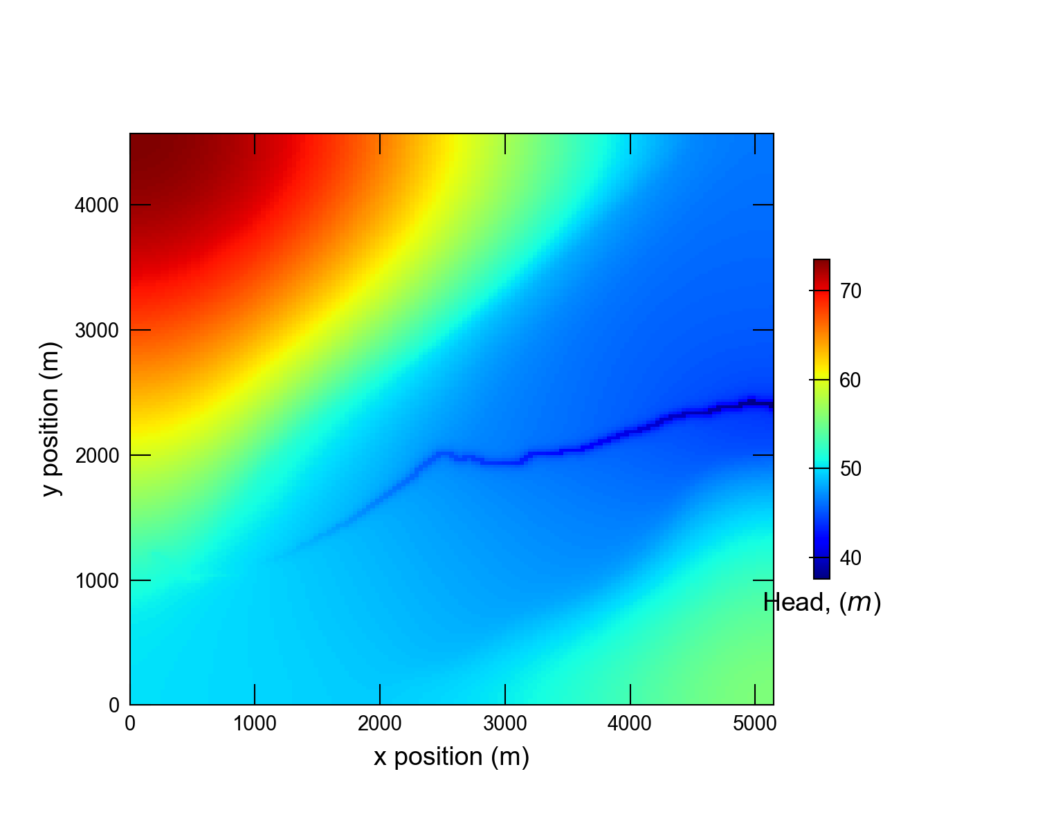
Figure 24.6 Simulated head in layer 1 for the GR model.
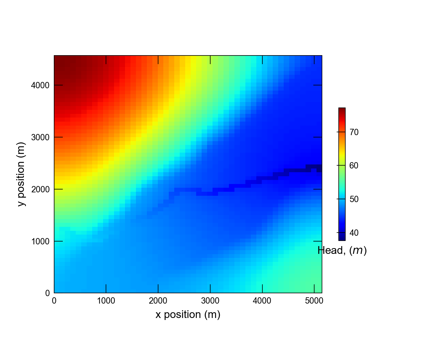
Figure 24.7 Simulated head in layer 1 for the GC model.
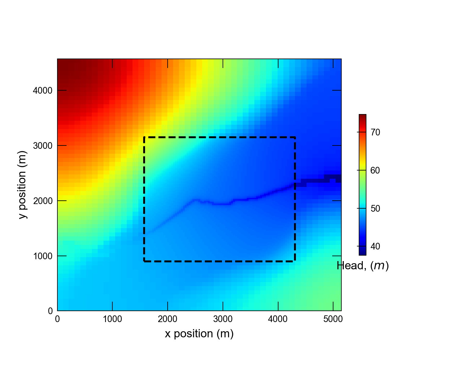
Figure 24.8 Simulated head in layer 1 for the LGR model. Dashed line indicates location of inset model with higher resolution than the outer coarse model.
24.3. References Cited
Vilhelmsen, T. N., Christensen, S., & Mehl, S. W. (2012). Evaluation of MODFLOW-LGR in connection with a synthetic regional-scale model. Groundwater, 50(1), 118–132. https://doi.org/10.1111/j.1745-6584.2011.00826.x
24.4. Jupyter Notebook
The Jupyter notebook used to create the MODFLOW 6 input files for this example and post-process the results is: