30. Capture Fraction Analysis

All groundwater pumped is balanced by removal of water somewhere, initially from storage in the aquifer and later from capture in the form of increase in recharge and decrease in discharge (Leake et al., 2010). Capture that results in a loss of water in streams, rivers, and wetlands now is a concern in many parts of the United States. Hydrologists commonly use analytical and numerical approaches to study temporal variations in sources of water to wells for select points of interest. Much can be learned about coupled surface/groundwater systems, however, by looking at the spatial distribution of theoretical capture for select times of interest. Development of maps of capture requires (1) a reasonably well-constructed transient or steady state model of an aquifer with head-dependent flow boundaries representing surface water features or evapotranspiration and (2) an automated procedure to run the model repeatedly and extract results, each time with a well in a different cell to evaluate the effect of a flux in a cell on an external boundary condition.

This example presents a streamflow capture analysis of the hypothetical aquifer system of (Freyberg, 1988) and based on the model datasets presented in (Hunt et al., 2020). The original problem of (Freyberg, 1988) documented an exercise where graduate students calibrated a groundwater model and then used it to make forecasts.

30.1. Example Description

A single-layer was used to simulate a shallow, water-table aquifer. The aquifer is surrounded by no-flow boundaries on the bottom and north-east-west sides (Figure 30.1). There is an outcrop area within the grid, where the water-table aquifer is missing. The aquifer is discretized using 40 rows and 20 columns (250 m on a side). A single steady-state stress period, with a single time step, was simulated. An arbitrary simulation period of 1 day was simulated. Model parameters for the example are summarized in Table 30.1.

The top of the model was set at an arbitrary elevation of 200 \(m\) (Table 30.1). The bottom elevations were not uniform; the aquifer was relatively flat on the east side and sloped gently to the south and west sides (see Hunt et al., 2020, fig. 1b). In the western area, and southeastern and southwestern corners of the aquifer, the impermeable bottom elevation was higher making for no-flow outcrop areas within the grid.

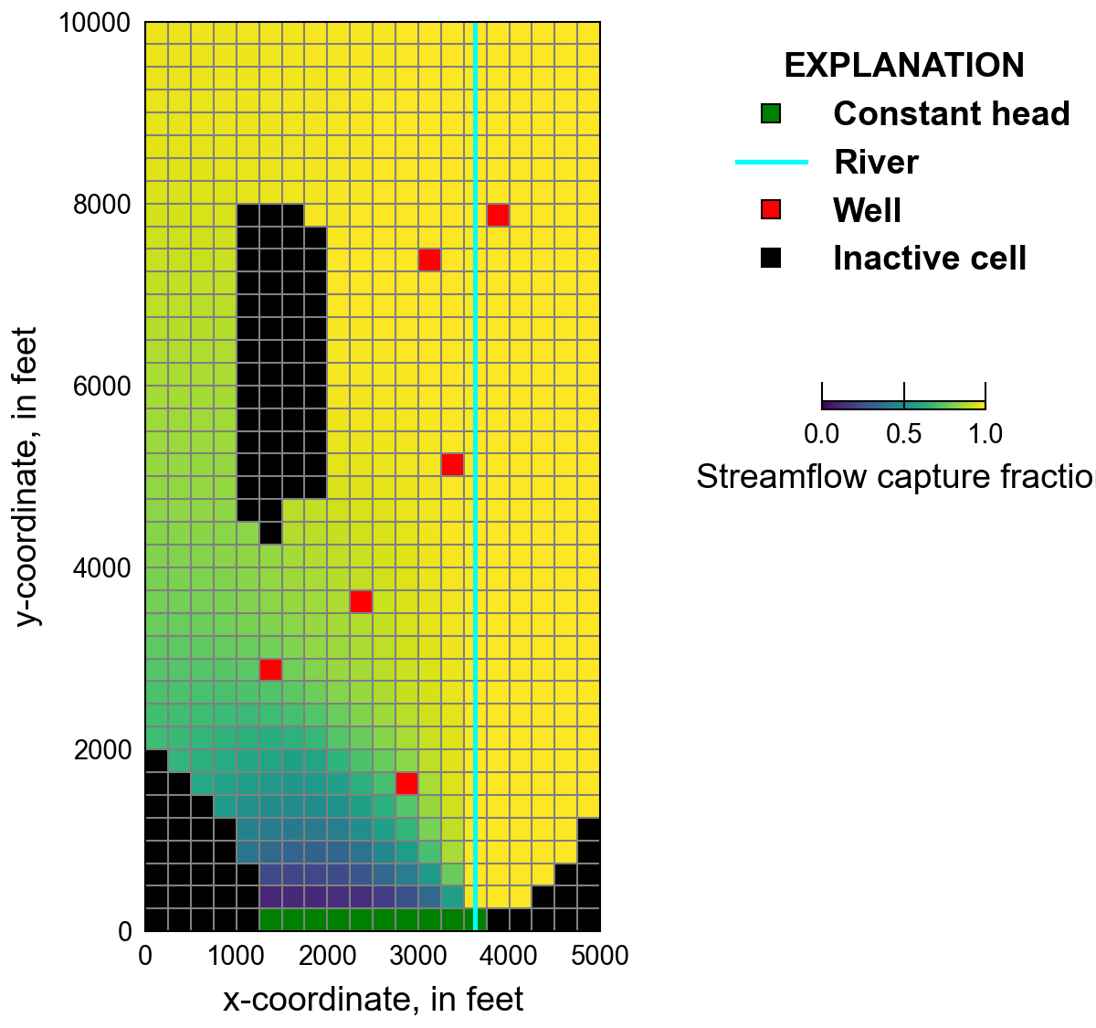
../_images/ex-gwf-capture-01.png — Figure 30.1 Diagram showing the model domain and the simulated streamflow capture fraction. The location of river cells, constant head cells, and wells are also shown.

Table 30.1 Model parameters for example ex-gwf-capture.
Parameter	Value
Number of periods	1
Number of layers	1
Number of rows	40
Number of columns	20
Column width (\(m\))	250.0
Row width (\(m\))	250.0
Top of the model (\(m\))	35.0
Cell conversion type	1
Starting head (\(m\))	45.0
Recharge rate (\(m/s\))	1.60000000e-09
Perturbation flux (\(m/s\))	–1e-3

Hydraulic conductivity (K) consisted of six zones (see Hunt et al., 2020, fig. 1c) with relatively small changes among them; areas of higher values of K were along the north, east and west boundaries, and adjacent to the western outcrop; K was lower in the south.

An initial head of 45 \(m\) is specified in each model cell. Flow into the system is from infiltration from precipitation and was represented using the recharge (RCH) package. A constant recharge rate of \(1 \times 10^{-9}\) \(m/s\) was specified for every active cell in the aquifer. A stream represented by river (RIV) package cells in column 15 in every row in the model and have river stages ranging from 20.1 \(m\) in row 1 to 11.25 \(m\) in row 40, a conductance of 0.05 \(m^2/s\), and bottom elevations ranging from 20 \(m\) in row 1 to 10.25 \(m\) in row 40 (Figure 30.1). River cells discharge groundwater from the model in every cells except river cells in row 9 and 10, which are a source of water for the model. Additional discharge of groundwater out of the model is from discharging wells represented by well (WEL) package cells and specified head cells. There are six pumping wells (Figure 30.1) with a total withdrawal rate of 22.05 \(m^3/s\). Heads are specified to be constant on the southern boundary in all active cells in row 40 and range from 16.9 \(m\) in column 6 to 11.4 \(m\) in column 15.

The Newton-Raphson formulation and Newton-Raphson under-relaxation were used to improve model convergence.

30.2. Example Results

The capture fraction analysis was performed using the MODFLOW Application Program Interface (API). An advantage of using the MODFLOW API is that model input files do not need to be regenerated. In this example, the streamflow capture fraction for a cell is calculated as

(30.1)\[ c_{k,i,j} = \frac{Q_{RIV}^{+} - Q_{{RIV}_{\text{base}}}}{|Q^{+}|} ,\]

where \(c_{k,i,j}\) is the streamflow capture fraction for an active cell (unitless), \(Q_{RIV}^{+}\) is the streamflow in the simulation with the perturbed flow in cell \((i,j,k)\) (\(L^3/T\)), \(Q_{{RIV}_{\text{base}}}\) is the streamflow in the base simulation (\(L^3/T\)), and \(Q^{+}\) is the flow that is added to an active cell (\(L^3/T\)).

Use of the MODFLOW API function requires replacement of the time-step loop in MODFLOW with an equivalent time-step loop in the programming language used to access in API. In this example, python is used to control MODFLOW. In addition to defining a replacement time-step loop, use of the MODFLOW API requires accessing program data in memory to control other programs being executed or to change MODFLOW data from the values defined in the MODFLOW input files.

When calculating the streamflow capture fraction, the specified flux in the second WEL package is set to the specified perturbation flux rate (Table 30.1) and the node number is modified to reduced node number for the cell being evaluated. The main loop that iterates over all of the active cells and adds the streamflow capture fraction to the appropriate location in the array used to store the values is listed below.

ireduced_node = -1
for irow in range(nrow):
    for jcol in range(ncol):

        # skip inactive cells
        if idomain[irow, jcol] < 1:
            continue

        # increment reduced node number
        ireduced_node += 1

        # calculate the perturbed river flow
        qriv = capture_fraction_iteration(mf6, cf_q, inode=ireduced_node)

        # add the value to the capture array
        capture[irow, jcol] = (qriv - qbase) / abs(cf_q)

The idomain array is a mapping array that identifies cells that have been removed from the simulation. The capture_fraction_iteration() function is listed below and returns the net stream flow (\(Q_{RIV}^{+}\)) after initializing the simulation (mobj.initialize()), adding the perturbation flux rate to the cell being evaluated (update_wel_pak()), running each time step in the simulation (mobj.update()), getting the net streamflow (get_streamflow()), and finalizing the simulation (mobj.finalize()).

def capture_fraction_iteration(mobj, q, inode=None):
    mobj.initialize()
    # time loop
    current_time = mobj.get_current_time()
    end_time = mobj.get_end_time()
    if inode is not None:
        update_wel_pak(mobj, inode, q)
    while current_time < end_time:
        mobj.update()
        current_time = mobj.get_current_time()
    qriv = get_streamflow(mobj)
    mobj.finalize()
    return qriv

The update_wel_pak() function is listed below and sets the number of boundaries (nbound) in the second WEL package to one, sets the perturbation location (nodelist) to the one-based reduced node number, and sets the specified flux rate (bound) to the perturbation flux value.

def update_wel_pak(mobj, inode, q):
    # set nbound to 1
    tag = mobj.get_var_address("NBOUND", sim_name, "CF-1")
    nbound = mobj.get_value(tag)
    nbound[0] = 1
    mobj.set_value(tag, nbound)
    # set nodelist to inode
    tag = mobj.get_var_address("NODELIST", sim_name, "CF-1")
    nodelist = mobj.get_value(tag)
    nodelist[0] = inode + 1  # convert from zero-based to one-based node number
    mobj.set_value(tag, nodelist)
    # set bound to q
    tag = mobj.get_var_address("BOUND", sim_name, "CF-1")
    bound = mobj.get_value(tag)
    bound[:, 0] = q
    mobj.set_value(tag, bound)

The get_streamflow() function gets the simulated flow between MODFLOW and the RIV Package and uses numpy to sum the flow for all of the RIV package cells into a net stream flow value (\(Q_{RIV}^{+}\)).

def get_streamflow(mobj):
    tag = mobj.get_var_address("SIMVALS", sim_name, "RIV-1")
    return mobj.get_value(tag).sum()

Simulated streamflow capture fraction results are shown in Figure 30.1. The stream captures all of the inflow to the model except west of the river in cells close to the constant head boundaries. Cells close to the western-most constant head boundary cells do not contribute any groundwater to the stream.

30.3. References Cited

Freyberg, D. L. (1988). An exercise in ground-water model calibration and prediction. Groundwater, 26(3), 350–360. https://doi.org/10.1111/j.1745-6584.1988.tb00399.x

Hunt, R. J., Fienen, M. N., & White, J. T. (2020). Revisiting “an exercise in groundwater model calibration and prediction” after 30 years: Insights and new directions. Groundwater, 58(2), 168–182. https://doi.org/10.1111/gwat.12907

Leake, S. A., Reeves, H. W., & Dickinson, J. E. (2010). A new capture fraction method to map how pumpage affects surface water flow. Groundwater, 48(5), 690–700. https://doi.org/10.1111/j.1745-6584.2010.00701.x

30.4. Jupyter Notebook

The Jupyter notebook used to create the MODFLOW 6 input files for this example and post-process the results is:

ex-gwf-capture