48. MT3DMS Supplemental Guide Problem 6.3.1
This example is for zero-order production in a uniform flow field. It is based on example problem 6.3.1 described in (Zheng, 2010). The problem consists of a one-dimensional model grid with inflow into the first cell and outflow through the last cell. This example is simulated with the GWT Model in MODFLOW 6, which receives flow information from a separate simulation with the GWF Model in MODFLOW 6. Results from the GWT Model are compared with the results from a MT3DMS simulation (Zheng, 1990) that uses flows from a separate MODFLOW-2005 simulation (Harbaugh, 2005).
48.1. Example description
The parameters used for this problem are listed in Table 48.1. The model grid consists of 101 columns, 1 row, and 1 layer. The flow problem is confined and steady state with an initial head set to the model top. The solute transport simulation represents transient conditions, which begin with an initial concentration specified as zero everywhere within the model domain. A specified flow condition is assigned to the first model cell. For the source pulse duration, the inflow concentration is specified as one. Following the source pulse duration the inflowing water is assigned a concentration of zero. A specified head condition is assigned to the last model cell. Water exiting the model through the specified head cell leaves with the simulated concentration of that cell.
Parameter |
Value |
|---|---|
Number of periods |
2 |
Number of layers |
1 |
Number of rows |
1 |
Number of columns |
101 |
Column width (\(m\)) |
0.16 |
Row width (\(m\)) |
1.0 |
Top of the model (\(m\)) |
1.0 |
Layer bottom elevation (\(m\)) |
0 |
Specific discharge (\(md^{-1}\)) |
0.1 |
Longitudinal dispersivity (\(m\)) |
1.0 |
Porosity of mobile domain (unitless) |
0.37 |
Zero-order production rate (\(mg/L d^{-1}\)) |
–2.0e-3 |
Source duration (\(d\)) |
160.0 |
Simulation time (\(t\)) |
840.0 |
Observation x location (\(m\)) |
8.0 |
48.2. Example Results
Simulated concentrations from the MODFLOW 6 GWT Model and MT3DMS are shown in Figure 48.1. The close agreement between the simulated concentrations demonstrate the zero-order-production capabilities implemented in the GWT Model.
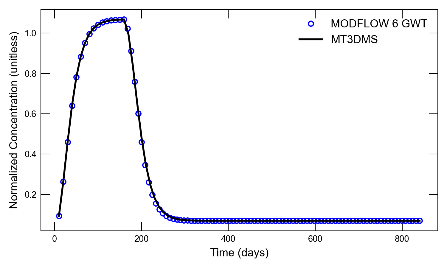
Figure 48.1 Concentrations simulated by the MODFLOW 6 GWT Model and MT3DMS for zero-order growth in a uniform flow field.
48.3. References Cited
Harbaugh, A. W. (2005). MODFLOW-2005, the U.S. Geological Survey modular ground-water model—the Ground-Water Flow Process. Retrieved from https://pubs.usgs.gov/tm/2005/tm6A16/
Zheng, C. (1990). MT3D, a modular three-dimensional transport model for simulation of advection, dispersion and chemical reactions of contaminants in groundwater systems.
Zheng, C. (2010). MT3DMS v5.3—a modular three-dimensional multi-species transport model for simulation of advection, dispersion and chemical reactions of contaminants in groundwater systems; supplemental user’s guide.
48.4. Jupyter Notebook
The Jupyter notebook used to create the MODFLOW 6 input files for this example and post-process the results is: