9. MODFLOW-NWT Problem 3
This example is based on problem 3 in (Niswonger et al., 2011) which used the Newton-Raphson formulation to simulate water levels in a rectangular, unconfined aquifer with a complex bottom elevation and receiving areally distributed recharge. This problem provides a good example of the utility of Newton-Raphson Formulation for solving problems with wetting and drying of cells.
9.1. Example Description
Model parameters for the example are summarized in Table 9.1.
Parameter |
Value |
|---|---|
Number of periods |
1 |
Number of layers |
1 |
Number of rows |
80 |
Number of columns |
80 |
Cell size in the x-direction (\(m\)) |
100.0 |
Cell size in y-direction (\(m\)) |
100.0 |
Top of the model (\(m\)) |
200.0 |
Horizontal hydraulic conductivity (\(m/day\)) |
1.0 |
Constant head water level (\(m\)) |
24.0 |
The model consists of a grid of 40 columns, 40 rows, and 1 layer. The model domain is 8,000 \(m\) in the x- and y-directions. The discretization is 100 \(m\) in the row and column direction for all cells. The top of the model is specified to be 200 \(m\) and the bottom of the model ranges from about 4 to 80 \(m\) (Figure 9.1). A single steady-state stress period, 365 days in length, with a single time step is simulated.
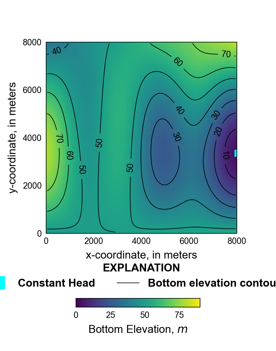
Figure 9.1 Distribution of layer-bottom elevations. The location of constant head boundary cells is also shown.
The horizontal hydraulic conductivity is 1 \(m/day\) and each cell is convertible. A initial head 20 \(m\) above the cell bottom was specified in all model cells.
Constant heads boundary condition cells with a specified value of 24 \(m\) are specified in column 80 for rows 46 through 48 (Figure 9.1). Recharge that is a function of the bottom elevation is specified for each active cells; two different recharge distributions are specified and are discussed further below.
Newton under-relaxation to maintain water-levels above the aquifer bottom (Hughes et al., 2017). The simple complexity Iterative Model Solver option and preconditioned bi-conjugate gradient stabilized linear accelerator was used for both scenarios.
9.2. Scenario Results
The model was evaluated using high and low recharge rates (Figure 9.2). Low recharge rates are 3 orders of magnitude less than the high recharge rates and simulate more arid conditions. Simulation results with large recharge rates are shown in Figure 9.3. The entire model domain is saturated and simulated saturated thickness ranges between zero and 25 \(m\) (Figure 9.3B). Simulation results with low recharge rates are shown in Figure 9.4. Only a small portion of the model domain has heads that are significantly above the cell bottom. However, all cells in the simulation have a non-zero saturated thickness (greater than 2 \(mm\)), which allows the applied recharge to flow horizontally toward the constant-head boundaries at the outlet of the aquifer.
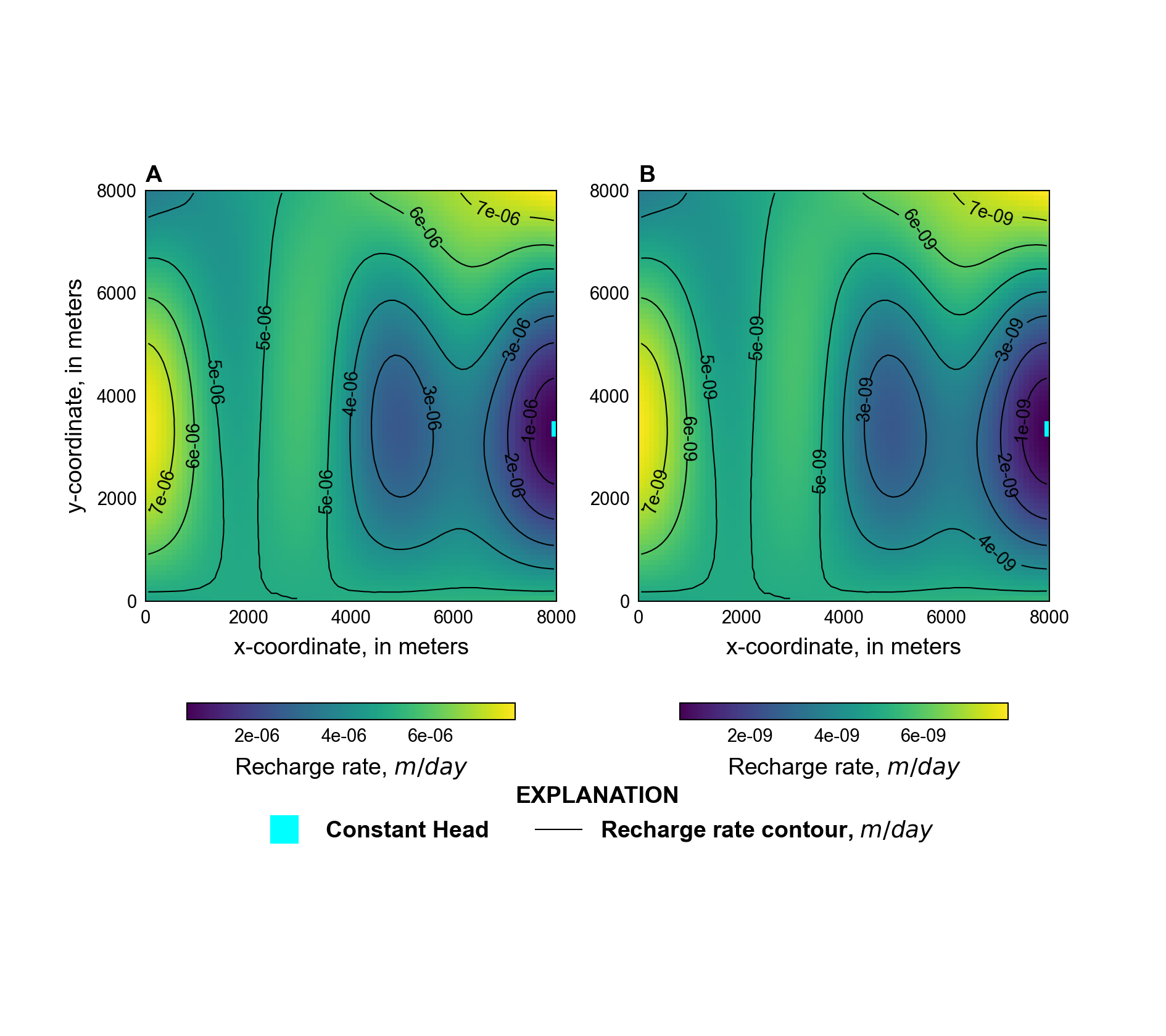
Figure 9.2 Distribution of groundwater recharge applied in the model scenarios. A, higher recharge rates, and B, lower recharge rates. The location of constant head boundary cells is also shown.
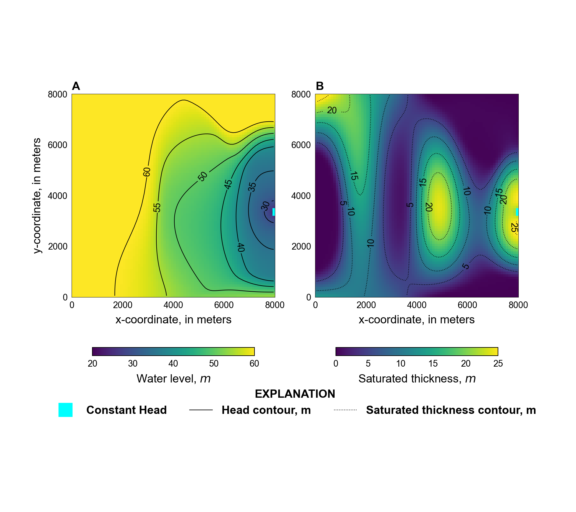
Figure 9.3 Distribution of heads and saturated thicknesses for the high recharge scenario. A, heads, and B, saturated thicknesses. The location of constant head boundary cells is also shown.
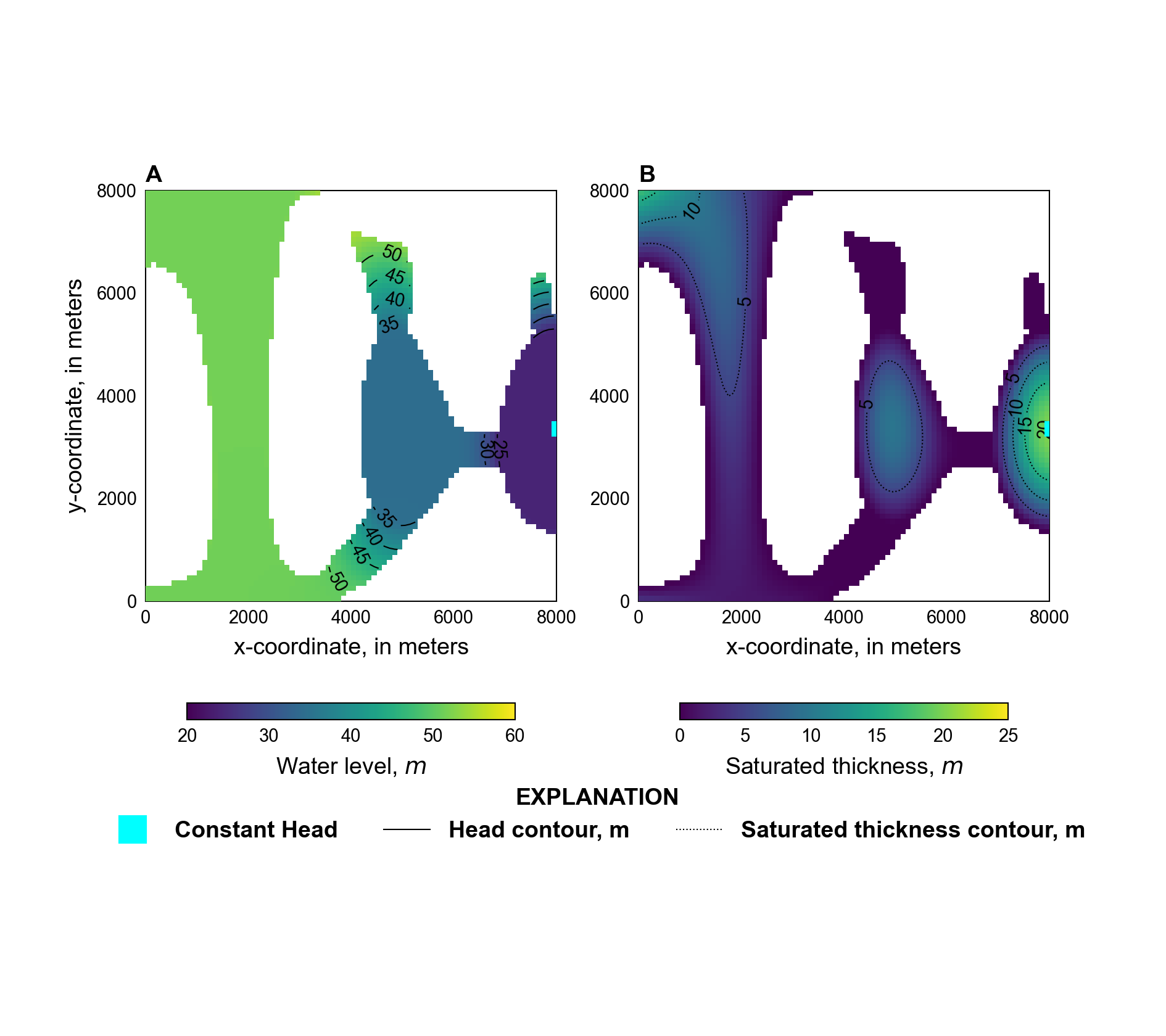
Figure 9.4 Distribution of heads and saturated thicknesses for the low recharge scenario. A, heads, and B, saturated thicknesses. The white regions indicate cells that have saturated thicknesses less than 1 \(mm\). The location of constant head boundary cells is also shown.
9.3. References Cited
Hughes, J. D., Langevin, C. D., & Banta, E. R. (2017). Documentation for the MODFLOW 6 framework. https://doi.org/10.3133/tm6A57
Niswonger, R. G., Panday, S., & Ibaraki, M. (2011). MODFLOW-NWT, A Newton formulation for MODFLOW-2005. Retrieved from https://pubs.er.usgs.gov/publication/tm6A37
9.4. Jupyter Notebook
The Jupyter notebook used to create the MODFLOW 6 input files for this example and post-process the results is: