18. Reilly Multi-Aquifer Well Problem
This is the unstressed multi-aquifer well simulation described in (Reilly et al., 1989). The example simulates a unconfined groundwater system that exhibits two-dimensional flow in vertical section and quantify the movement of water through a well under nonpumping conditions.
18.1. Example Description
A two-dimensional cross-section model was developed to provide lateral boundary conditions for a local scale model that included the effects of a nonpumping well screened across multiple model layers. The multi-aquifer well was represented using a multi-aquifer well and a vertical string of high hydraulic conductivity cells in order to compare multi-aquifer well results to the results of (Reilly et al., 1989). Model parameters for the regional and local model examples are summarized in Table 18.1.
Parameter |
Value |
|---|---|
Number of periods |
1 |
Number of layers (regional) |
21 |
Number of rows (regional) |
1 |
Number of columns (regional) |
200 |
Number of layers (local) |
41 |
Number of rows (local) |
16 |
Number of columns (local) |
27 |
Regional column width (\(ft\)) |
50.0 |
Regional row width (\(ft\)) |
1.0 |
Top of the model (\(ft\)) |
10.0 |
Model bottom elevation (\(ft\)) |
–205.0 |
Starting head (\(ft\)) |
10.0 |
Horizontal hydraulic conductivity (\(ft/d\)) |
250.0 |
Vertical hydraulic conductivity (\(ft/d\)) |
50.0 |
Areal recharge (\(ft/d\)) |
0.004566 |
Regional downgradient constant head (\(ft\)) |
0.0 |
Row, column location of well |
(15, 13) |
Layers with well screen |
(1, 12) |
Well radius (\(ft\)) |
0.1333 |
Bottom of the well (\(ft\)) |
–65.0 |
Hydraulic conductivity for well (\(ft/d\)) |
1e9 |
18.1.1. Regional Model
The regional model consists of a grid of 200 columns, 1 row, and 21 layers. The model domain is 10,000 and 1 \(ft\) in the x- and y-directions (Figure 18.1). The discretization is in the column directions is 50 \(ft\). The top of the model is specified to be 10 \(ft\) and the bottom of the aquifer is specified to be -205 \(ft\). The bottom of the first model layer is -5 \(ft\) and layers 2 through 21 are 10 \(ft\) thick. A single steady-state stress period 1 day in length is simulated. The stress period has 1 time step.
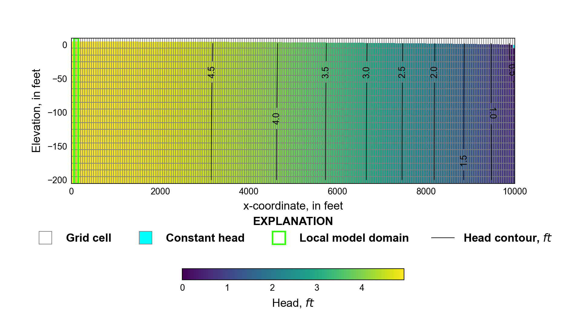
Figure 18.1 Diagram showing the regional cross-section model with the location of the local three-dimensional model simulating flow through a wellbore. Steady-state water-table elevation and heads along with the location of the downgradient constant head boundary.
The horizontal and vertical hydraulic conductivity is 250 and 50 \(ft/d\). The upper model layer was specified to be convertible (unconfined) and all other model layers are specified to be confined. An initial head of 10 \(ft\) is specified, but any value above the bottom of each layer could have been specified since the simulation is steady state.
Flow into the system is from infiltration from precipitation and was represented using the recharge (RCH) package. A constant recharge rate of \(4.566 \times 10^{-3}\) \(ft/d\) (20 \(in/yr\)) was specified for every cell in model layer 1. Flow out of the model is from a specified downgradient outflow boundary represented by a constant head (CHD) package cells in model layer 1.
18.1.2. Local Model
Since the flow system is symmetric around the well, only half of the local domain was simulated. The local model consists of a grid of 27 columns, 16 rows, and 41 layers. The model domain is 100 and 50 \(ft\) in the x- and y-directions (Figure 18.2). The discretization is in the column and row directions, ranging from 10 to 0.1665 \(ft\). In the cell containing the well (row 16, column 14) the discretization is 0.333 and 0.1665 \(ft\) (4 and 2 \(in\)) in the x- and y-directions, respectively. The top of the model is specified to be 10 \(ft\) and the bottom of the aquifer is specified to be -205 \(ft\). The bottom of the first model layer is -5 \(ft\) and layers 2 through 41 are 5 \(ft\) thick. A single steady-state stress period 1 day in length is simulated. The stress period has 1 time step.
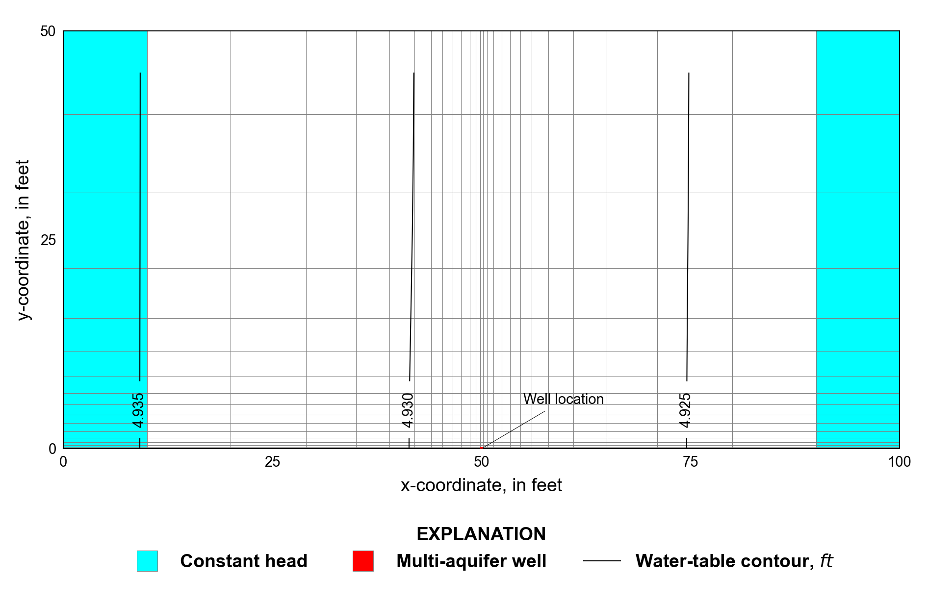
Figure 18.2 Diagram showing the horizontal discretization used in the local three-dimensional model simulating flow through a wellbore. Steady-state water-table contours are shown along with the location of the multi-aquifer well and constant head boundaries.
The horizontal and vertical hydraulic conductivity is 250 and 50 \(ft/d\). The upper model layer was specified to be convertible (unconfined) and all other model layers are specified to be confined. An initial head of 10 \(ft\) is specified, but any value above the bottom of each layer could have been specified since the simulation is steady state.
Flow into the system is from infiltration from precipitation and was represented using the recharge (RCH) package. A constant recharge rate of \(4.566 \times 10^{-3}\) \(ft/d\) (20 \(in/yr\)) was specified for every cell in model layer 1. Simulated regional results were used to define constant head values specified in columns 1 and 27. The heads in column 1 and 2 of the regional model were linearly interpolated to the node position in column 1 to define constant heads in the first column of the local model. The heads in column 3 and 4 of the regional model were linearly interpolated to the node position in column 27 to define constant heads in the last column of the local model. Vertically, linearly interpolated heads from layer 2 through 21 in the regional model were applied to the two equivalent layers in the local model.
The well is located in the lower center of the model domain (Figure 18.2), has a 60 \(ft\) screened interval that fully penetrates model layers 2 through 13, has a well radius of 0.1333 \(ft\), the well bottom is at -65 \(ft\), and is not pumping. In order to compare results to a version of the local model that simulated the well using high hydraulic conductivity the well is located in (row 16, column 14) but physically connected to the three cells horizontally connected to the cell. Furthermore, the top and bottom of the well are connected to the overlying and underlying cells in layer 1 and layer 14.
The conductance for each connection was calculated using the same harmonic average used by MODFLOW 6 to calculate intercell conductance (see Langevin et al., 2017, pp. eq.4–24). The equivalent hydraulic conductivity of the cell containing the well is based on the Hagen-Poiseuille equation for laminar pipe flow by an equivalent form of Darcy’s law and is used in MODFLOW 6. For laminar flow, the Hagen-Poiseuille equation is
where \(Q_{pipe}\) is the flow through the pipe (in this case wellbore) (L\(^{3}\)/T), \(V\) is the velocity (L/T), \(A\) is the cross-sectional area of the pipe (L\(^{2}\)), \(d\) is the diameter of the pipe (L), \(g\) is the acceleration due to gravity (L/T\(^{2}\)), \(\nu\) is the kinematic viscosity of the flowing fluid (L\(^{2}\)/T), and \(\Delta h\) is the head loss (L). Darcy’s law is
where \(Q\) is the flow through a block of porous medium, \(K\) is the hydraulic conductivity of the medium (L/T), and \(L\) is the length of flow section (L). The equivalent hydraulic conductivity (\(K_{eq}\)) representing the wellbore can be calculated by equating equations 18.1 and 18.2 and rearranging to solve for \(K_{eq}\). The equivalent hydraulic conductivity is
A total of 38 multi-aquifer well connections to the connected aquifer were defined and had conductances values equal to 1.11 (connections to layer 1 and 14), 832.50 (connections to column 13 and 15 in layers 2 through 13), and 3330.000 \(ft^{2}/d\) (connection to row 15 in all layers). The initial head in the well was set equal to the initial head in the aquifer (10.0 \(ft\)). For the case where the well represented as a multi-aquifer well, the cell in row 16, column 14, and layers 2 through 13 was inactivated by specifying an IDOMAIN value of 0 in these cells. For the case where the well was represented using high hydraulic conductivity, the horizontal and vertical hydraulic conductivity in row 16, column 14, and layers 2 through 13 was set to \(1 \times 10^{9}\) \(ft/d\) (see eq. 18.3).
18.2. Example Results
Steady-state results for the regional model are shown in Figure 18.1. Steady-state water-table elevations for the local three-dimensional model with the well simulated using a multi-aquifer well are shown in Figure 18.2. The flow with depth into or from the wellbore is shown in Figure 18.3. The flow to or from the wellbore for the case where the multi-aquifer well and high hydraulic conductivity were used is in close agreement and the mean error for all of the cells connected to the wellbore is \(-2.14 \times 10^{-6}\) \(ft^{3}/d\). The total flow into and out of the wellbore is 9.53 and 9.52 \(ft^{3}/d\) for the case with the multi-aquifer well and high hydraulic conductivity, respectively. The steady-state head in the wellbore and the average head for all cells representing the well in the high hydraulic conductivity case are both 4.93 \(ft\).
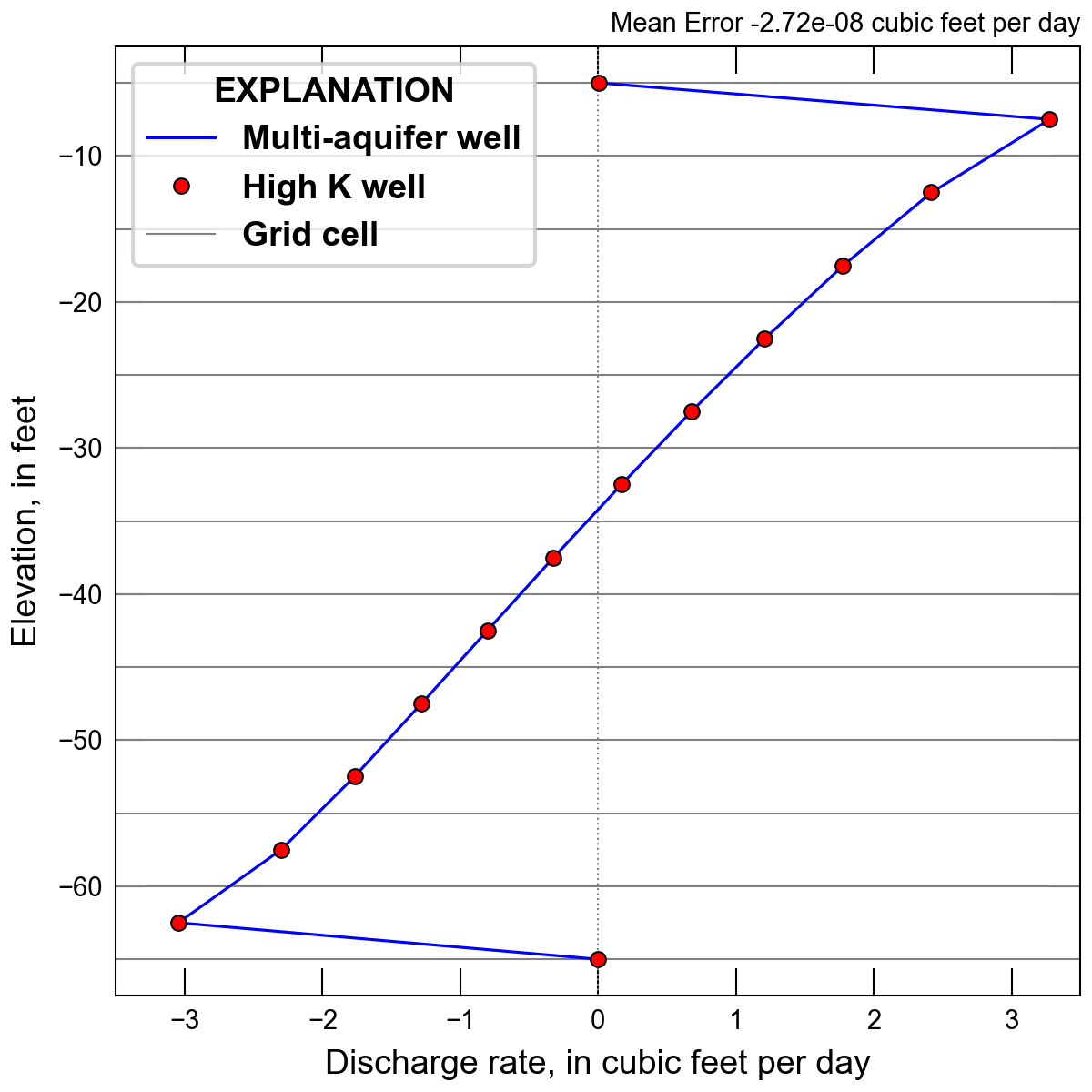
Figure 18.3 Graph of flow between the aquifer and the borehole with depth for the three-dimensional local model with the well represented as a multi-aquifer well and using high hydraulic conductivity. Positive discharge values indicate flow from the aquifer to the wellbore. Negative discharge values indicate flow from the wellbore to the aquifer.
18.3. References Cited
Langevin, C. D., Hughes, J. D., Provost, A. M., Banta, E. R., Niswonger, R. G., & Panday, S. (2017). Documentation for the MODFLOW 6 Groundwater Flow (GWF) Model. https://doi.org/10.3133/tm6A55
Reilly, T. E., Franke, O. L., & Bennett, G. D. (1989). Bias in groundwater samples caused by wellbore flow. Journal of Hydraulic Engineering, 115(2), 270–276. https://doi.org/10.1061/(ASCE)0733-9429(1989)115:2(270)
18.4. Jupyter Notebook
The Jupyter notebook used to create the MODFLOW 6 input files for this example and post-process the results is: