40. MT3DMS Problem 4
The third demonstrated MT3DMS-MODFLOW 6 transport comparson is for a two-dimensional transport in a diagonal flow field. This problem is similar to the preceding problem with two important changes. First, the flow direction is now oriented at a 45-degree angle relative to rows and columns of the numerical grid. Owing the use of MT3DMS for comparison, the MODFLOW 6 solution uses the traditional DIS package (not DISU or DISV). The second notable change is that the number of rows and columns has been expanded in order to accommodate a longer simulation period of 1,000 days. Because of the orientation of the flow field relative to the model grid, and the sharpness of the migrating concentration front, this test problem presents a challenging set of conditions to simulate. Three scenarios test alternative advection formulations, as summarized in Table 40.1
Scenario |
Scenario Name |
Parameter |
Value |
|---|---|---|---|
1 |
ex-gwt-mt3dms-p04a |
mixelm (unitless) |
0 |
2 |
ex-gwt-mt3dms-p04b |
mixelm (unitless) |
-1 |
3 |
ex-gwt-mt3dms-p04c |
mixelm (unitless) |
1 |
Model parameter values for this problem are provided in Table 40.2.
Parameter |
Value |
|---|---|
Number of layers |
1 |
Number of rows |
100 |
Number of columns |
100 |
Column width (\(m\)) |
10.0 |
Row width (\(m\)) |
10.0 |
Layer thickness (\(m\)) |
1.0 |
Top of the model (\(m\)) |
0.0 |
Porosity |
0.14 |
Simulation time (\(days\)) |
365 |
Horizontal hydraulic conductivity (\(m/d\)) |
1.0 |
Volumetric injection rate (\(m^3/d\)) |
0.01 |
Concentration of injected water (\(mg/L\)) |
1000.0 |
Longitudinal dispersivity (\(m\)) |
2.0 |
Ratio of transverse to longitudinal dispersitivity |
0.1 |
Molecular diffusion coefficient (\(m^2/d\)) |
1.0e-9 |
The same analytical solution used in the previous problem can be used for this problem after applying the necessary updates to select parameters - most notably the dispersion and porosity terms and that an inter-model comparison is drawn after 1,000 days instead of 365 days. Figure 36 in (Zheng & Wang, 1999) shows four different solutions for this problem: (1) analytical, (2) Method of Characteristics (MOC), (3) upstream finite difference (FD), and (4) Total Variation Dimishing (TVD) or “ULTIMATE” scheme. Both the MOC and TVD solutions demonstrate a reasonable agreement with the analytical solution. However, the upstream finite difference solution reflects considerably more spread from simulation of too much dispersion - in this case numerical dispersion instead of hydrodynamic dispersion.
The MODFLOW 6 transport solution is compared to all three numerical solutions (FD, TVD, and MOC) presented in (Zheng & Wang, 1999). The first comparison shows complete agreement between MT3DMS and the MODFLOW 6 transport solution when the finite difference approach is applied (Figure 40.1).
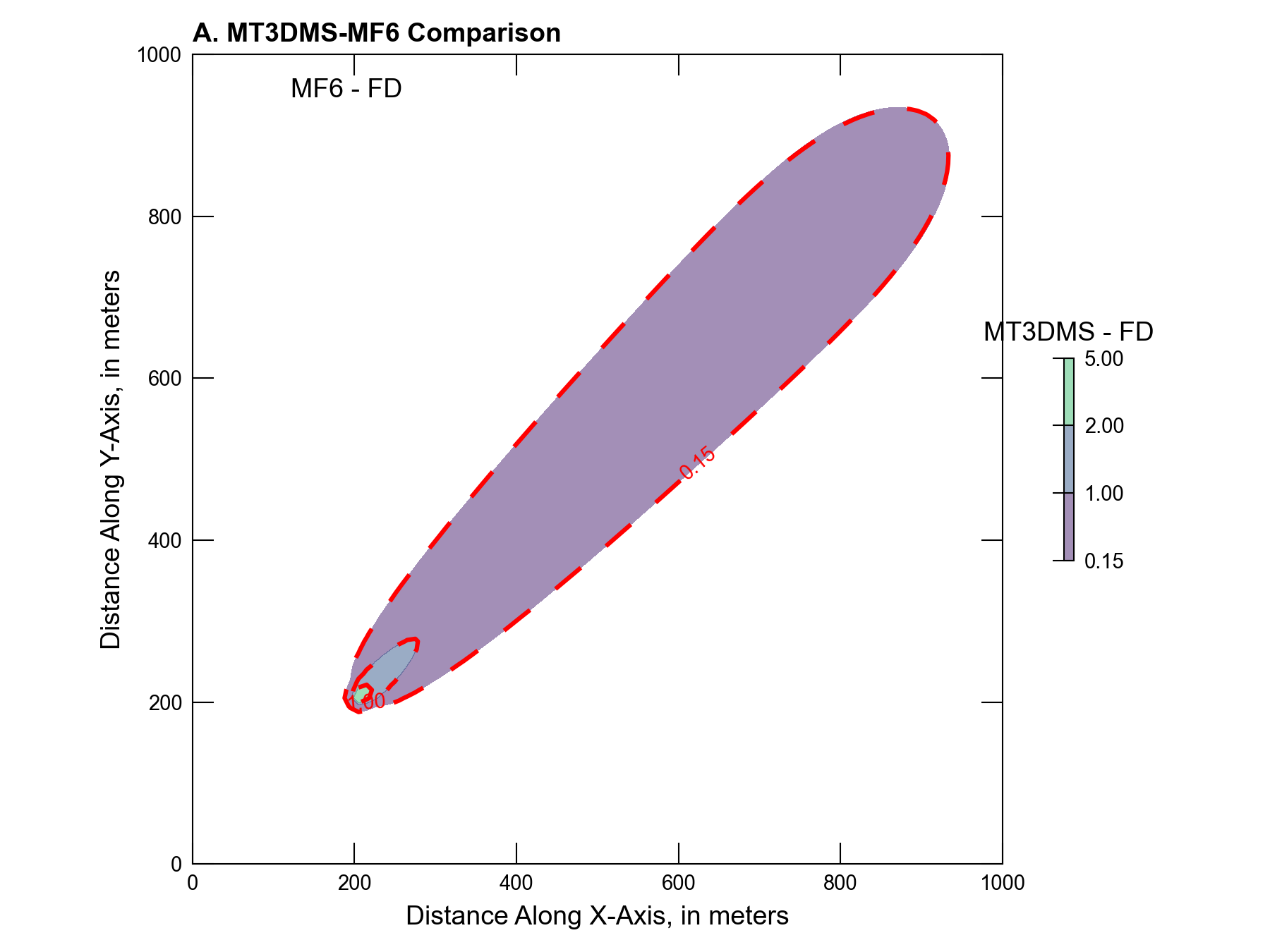
Figure 40.1 Comparison of the MT3DMS and MODFLOW 6 numerical solutions for two-dimensional transport in a diagonal flow field. Both models are using their respective finite difference solutions without the TVD option
Figure 40.2 shows a comparison between the MT3DMS and MODFLOW 6 solution with the respective TVD options for each model activated. Owing to the fact that MT3DMS uses a third-order TVD scheme while MODFLOW 6 uses a second-order scheme, differences between the two solutions are expected.
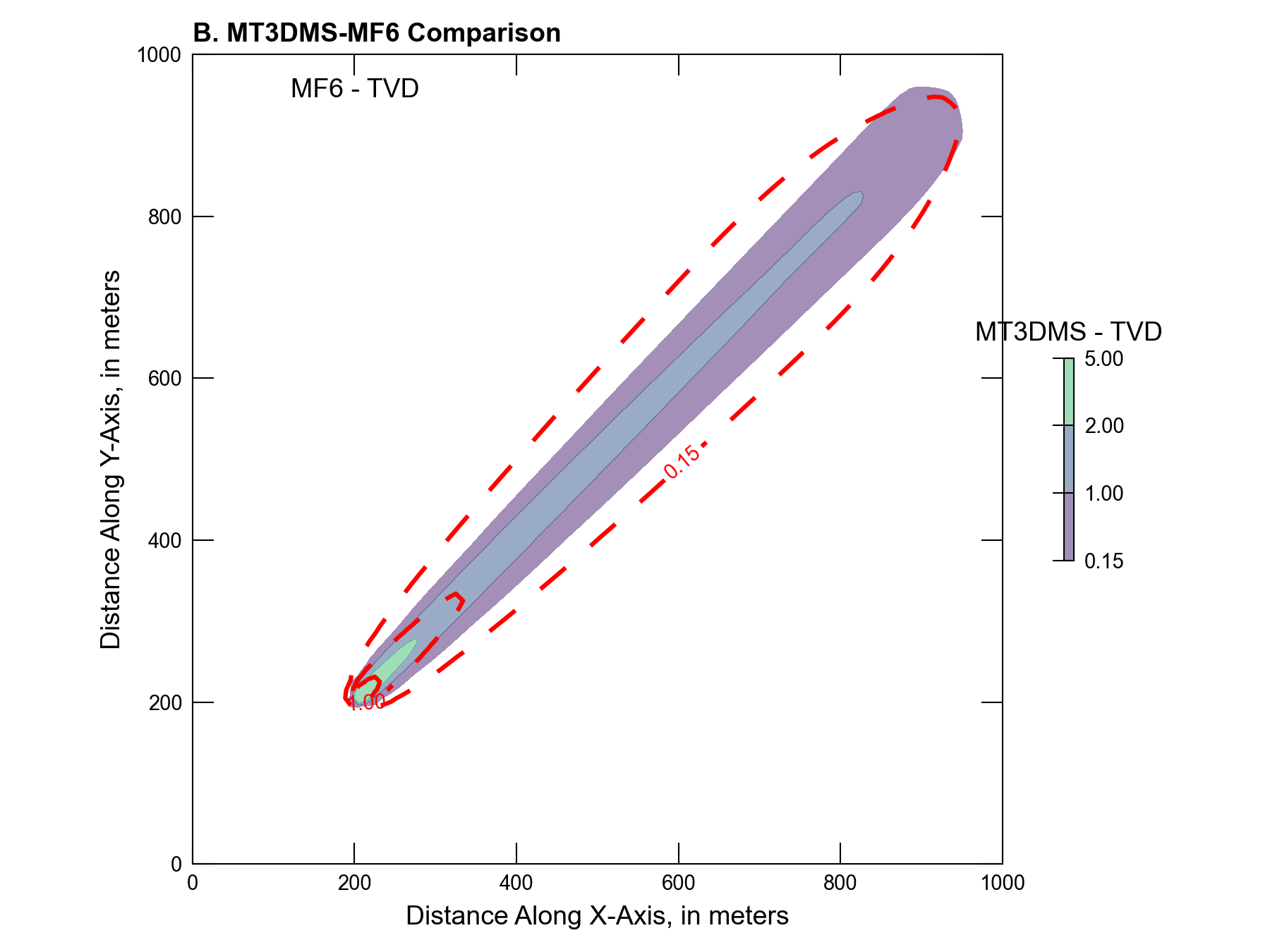
Figure 40.2 Comparison of the MT3DMS and MODFLOW 6 numerical solutions for two-dimensional transport in a diagonal flow field. Both models are using their respective finite difference solutions with the use of the TVD option, which serves as the main difference with results displayed in Figure 40.2
The third model comparison shows the largest difference between the two solutions (Figure 40.3). Because the MOC solution is the closest facsimile of the analytical solution, comparison of MODFLOW 6 with the MT3DMS MOC solution is as close to a comparison with the analytical solution as will be shown for the current set of model runs.
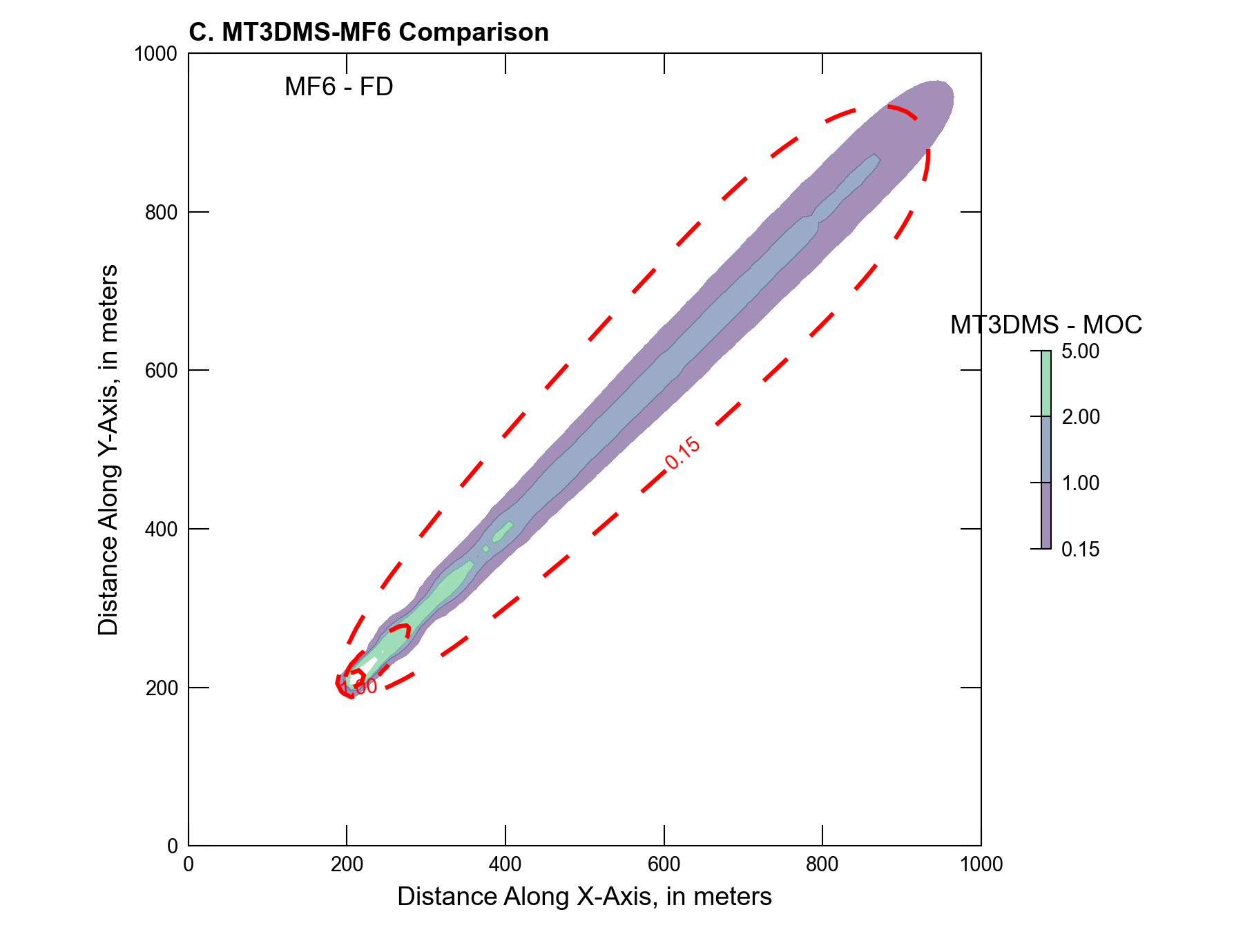
Figure 40.3 Comparison of the MT3DMS and MODFLOW 6 numerical solutions for two-dimensional transport in a diagonal flow field. Here, MT3DMS is using a MOC technique to find a solution while MODFLOW 6 uses finite difference without TVD activated.
40.1. References Cited
Zheng, C., & Wang, P. P. (1999). MT3DMS—a modular three-dimensional multi-species transport model for simulation of advection, dispersion and chemical reactions of contaminants in groundwater systems; documentation and user’s guide.
40.2. Jupyter Notebook
The Jupyter notebook used to create the MODFLOW 6 input files for this example and post-process the results is: