6. Nested Grid Problem - Two Domains

This example reproduces the nested grid problem described in the MODFLOW-USG documentation (Panday et al., 2013). A single model setup with a grid based on the Discretization by Vertices (DISV) input is presented elsewhere in these examples. This problem is set up using two individual GWF models with a regular grid (DIS) that are coupled through a GWF Exchange. A plan view of the combined grid for the two models is shown in Figure 6.1. The XT3D option in the NPF package can be applied to avoid inaccuracies at the cell refinement interface (Provost et al., 2017), which is the model boundary in this example. However, for this coupled system it is not sufficient to enable XT3D for the models independently: the correct flow calculation around the model interface relies on information from both models.

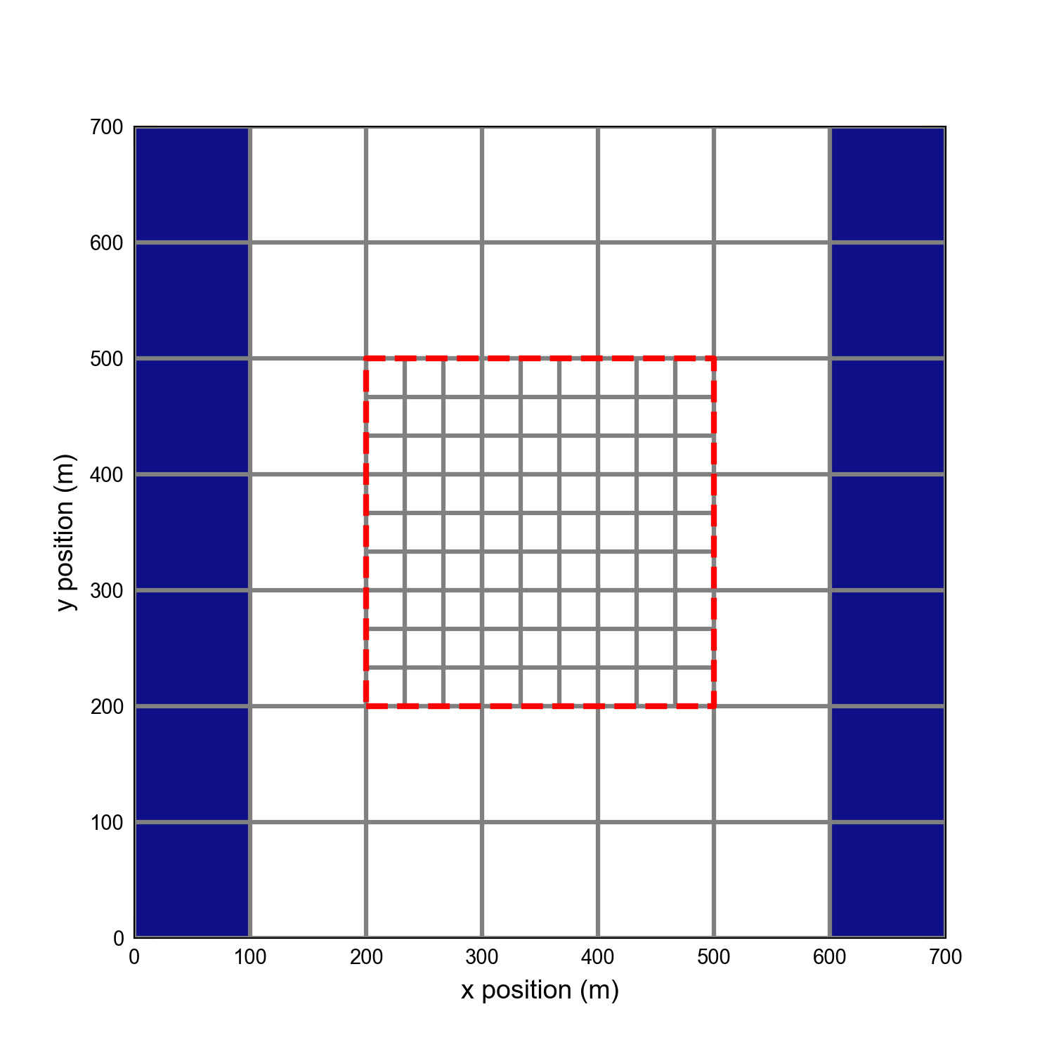
Figure 6.1 A top view of the grids of the outer and inner model used in this example. The dashed red line indicates the interface between the two. The blue shaded areas are the cells with a constant head boundary condition.

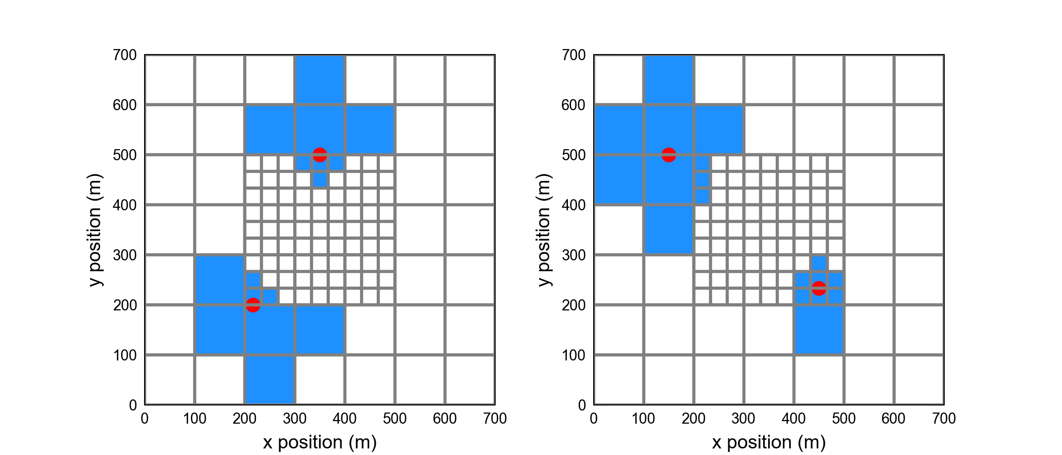
Figure 6.2 Flow calculation stencils for XT3D for the coupled model system. Details in the text.

This is illustrated in more detail in Figure 6.2. The red dots show (examples of) cell connections where the flow relies on data from both models. The cells which are involved in the flow calculation are colored blue. In the left panel this is the case for flows that cross the model boundary. On the right it is shown how interior connections can still be dependent on cell data from the neighboring model. With the release of the generalized coupling framework in MODFLOW 6(as of version 6.3.0) it is now possible to activate XT3D not just for the internal model connections, but also for connections between models. Additionally, it will correctly calculate the XT3D fluxes near the model boundary using data from both models (c.f. the right panel in Figure 6.2). In this example problem we study how these options affect the accuracy of the simulation results.

6.1. Example Description

This is a typical Local Grid Refinement (LGR) example with the coarse outer cells (\(100 m \times 100 m\)) being part of one model and the refined inner cells part of the other. Some essential and uniform parameters are given in Table 6.1. The two models are connected by a GWF Exchange which enables groundwater flow through the grid faces marked by the dashed red square. The blue cells indicate where a constant head boundary condition is imposed. The condition is set to 1\(m\) for the cells on the left and to 0\(m\) for the right. As a result, the analytical solution of the problem is trivial and given by the expression

(6.1)\[h = 1.0 - \frac{x - 50.0}{600.0} m\]

for the head \(h\) and \(x \in (50.0,650.0)\). This formula will be used to test the accuracy of the simulated results presented below.

Table 6.1 Model parameters for example ex-gwf-u1gwfgwf.

Parameter	Value
Number of periods	1
Number of layers	1
Top of the model (\(m\))	0.0
Layer bottom elevations (\(m\))	–100.0
Starting head (\(m\))	0.0
Constant head boundary LEFT (\(m\))	1.0
Constant head boundary RIGHT (\(m\))	0.0
Cell conversion type	0
Horizontal hydraulic conductivity (\(m/d\))	1.0

6.2. Scenario Results

The nested grid problem was run for 4 different scenarios using the parameter configuration listed in Table 6.2.

Table 6.2 Scenario parameters for example ex-gwf-u1gwfgwf.

Scenario	Scenario Name	Parameter	Value
1	ex-gwf-u1gwfgwf-s1	XT3D in models	False
		XT3D at exchange	False
2	ex-gwf-u1gwfgwf-s2	XT3D in models	True
		XT3D at exchange	False
3	ex-gwf-u1gwfgwf-s3	XT3D in models	True
		XT3D at exchange	True
4	ex-gwf-u1gwfgwf-s4	XT3D in models	False
		XT3D at exchange	True

Model results for the simulation of these scenarios are shown in Figure 6.3, Figure 6.4, Figure 6.5, Figure 6.6. Flow is from left to right and should be perfectly one-dimensional. The head surface should represent a flat plane with a value of 1.0 on the left and zero on the right, following the analytical expression given in equation 6.1.

Because the configuration of a nested grid with a refinement violates the control-volume finite-difference assumptions, there are errors in the simulated heads for scenario 1 with the standard NPF flow formulation, as shown in Figure 6.3B. Enabling the XT3D method in both models as done in scenario 2, is insufficient to get rid of these accuracies as can be seen from Figure 6.4B. Scenario 3 applies the advanced XT3D calculation globally on both models and at the interface. This setup is now equivalent to what was presented in the “Nested Grid Problem” elsewhere in these examples for the case of a single DISV-based model with XT3D enabled. And as expected, Figure 6.5B illustrates how in this case the deviation from the analytical result is well within the solver tolerance (\(h_\textrm{close}=1 \times 10^{-9}\)). Scenario 4 is a new capability of the generalized coupling and allows to apply XT3D where it is needed: in the exchange region between the models (c.f. Figure 6.2B). Because the XT3D calculation is quite costly, this is an efficient alternative to the setup in scenario 3 which leads to the same level of accuracy. The latter is clearly demonstrated by the error plot in Figure 6.6B.

Figure 6.3 Results for scenario 1: simulated head (A) and differences in head with respect to the analytical result (B) for a system of coupled models without XT3D.

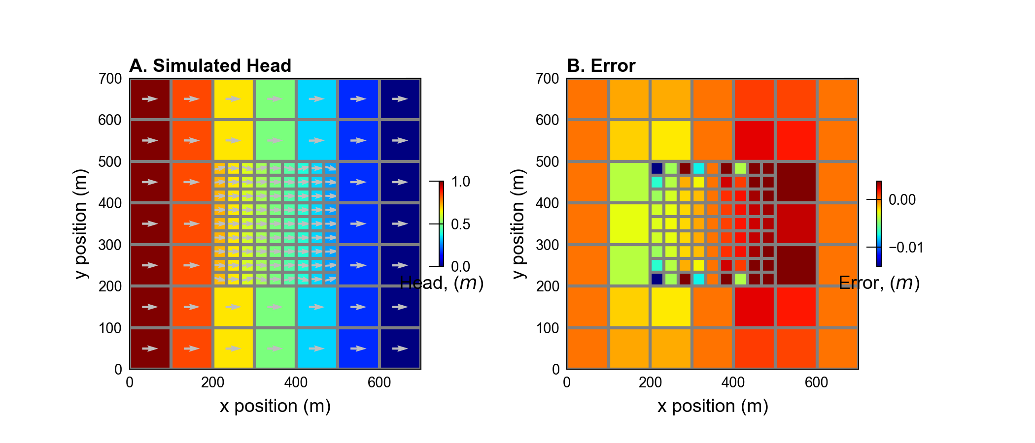
Figure 6.4 Results for scenario 2: simulated head (A) and differences in head with respect to the analytical result (B) for a system of coupled models with XT3D active in both models but not at the exchange between them.

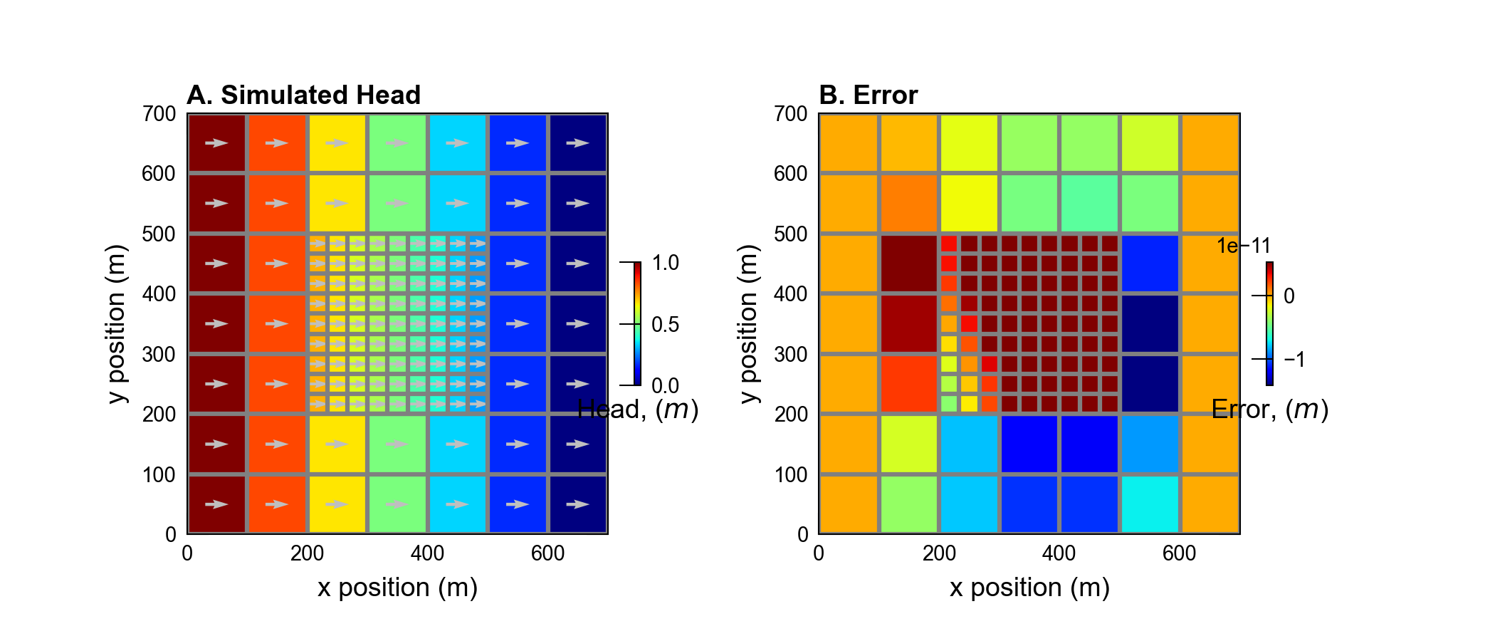
Figure 6.5 Results for scenario 3: simulated head (A) and differences in head with respect to the analytical result (B) for a system of coupled models with XT3D active in both models and at the exchange between them.

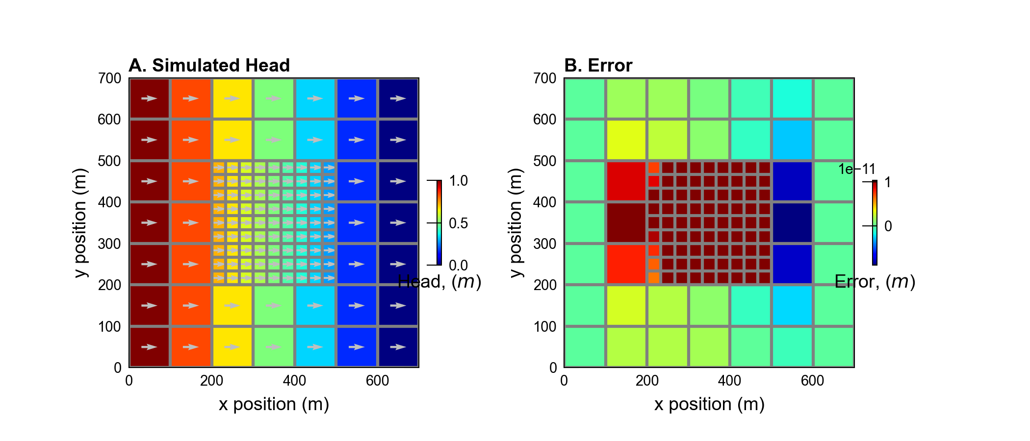
Figure 6.6 Results for scenario 4: simulated head (A) and differences in head with respect to the analytical result (B) for a system of coupled models without XT3D in the models but with XT3D enabled at the exchange between them.

6.3. References Cited

Panday, S., Langevin, C. D., Niswonger, R. G., Ibaraki, M., & Hughes, J. D. (2013). MODFLOW-USG version 1—an unstructured grid version of MODFLOW for simulating groundwater flow and tightly coupled processes using a control volume finite-difference formulation. Retrieved from https://pubs.usgs.gov/tm/06/a45/

Provost, A. M., Langevin, C. D., & Hughes, J. D. (2017). Documentation for the “XT3D” Option in the Node Property Flow (NPF) Package of MODFLOW 6. https://doi.org/10.3133/tm6A56

6.4. Jupyter Notebook

The Jupyter notebook used to create the MODFLOW 6 input files for this example and post-process the results is:

• ex-gwf-u1gwfgwf