8. MODFLOW-NWT Problem 2
This example is based on problem 2 in (Niswonger et al., 2011) which used the Newton-Raphson formulation to simulate dry cells under a recharge pond. This problem is also described in (McDonald et al., 1992) and used the MODFLOW rewetting option to rewet dry cells.
8.1. Example Description
The simulation represents a rectangular, unconfined aquifer with a deep water table. The model uses symmetry to simplify the problem by simulating one-quarter of the pond and the downgradient model domain (Figure 8.1). Model parameters for the example are summarized in Table 8.1
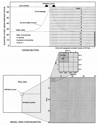
Figure 8.1 Hydrogeology, model grid, and model boundary conditions (from McDonald et al., 1992).
The model consists of a grid of 40 columns, 40 rows, and 14 layers. The model domain is 5,000 \(ft\) in the x- and y-directions. The discretization is 125 \(ft\) in the row and column direction for all cells. The upper model layer is 15 \(ft\) thick and the remaining model layers (layers 2 through 14) are 5 \(ft\) thick. Four stress periods are simulated. The first three stress periods are transient and the last stress period is steady state. The stress periods are 190, 518, 1921, and 1 days in length and are broken up into 10, 2, 17, and 1 time steps of equal length. The total simulation time at the end of the four stress periods are 190, 708, 2,630, and 2,631 days, respectively.
Parameter |
Value |
|---|---|
Number of periods |
4 |
Number of layers |
14 |
Number of rows |
40 |
Number of columns |
40 |
Column width (\(ft\)) |
125.0 |
Row width (\(ft\)) |
125.0 |
Top of the model (\(ft\)) |
80.0 |
Horizontal hydraulic conductivity (\(ft/day\)) |
5.0 |
Horizontal hydraulic conductivity (\(ft/day\)) |
0.25 |
Specific storage (\(1/day\)) |
0.0002 |
Specific yield (unitless) |
0.2 |
Constant head along left and lower edges and starting head (\(ft\)) |
25.0 |
Recharge rate (\(ft/day\)) |
0.05 |
The horizontal hydraulic conductivity is 5 \(ft/day\) and vertical hydraulic conductivity is 0.25 \(ft/day\). The upper ten model layers are convertible and the lower four model layers are confined. The specific yield is 0.2 (unitless) and the specific storage is 0.0002 \(1/day\). Unconfined and confined storage change is simulated in the upper ten model layers; confined storage change is simulated the lower four model layers.
A initial head of 25 \(ft\) was specified in all model cells, which results in the upper 9 model layers being dry at the start of the simulation. Constant heads boundary condition cells with a specified value of 25 \(ft\) were specified on the right and lower edges of the model in model layer 10 through 14. The pond area above the aquifer is approximately 6 acres and recharge is added to four cells in the upper left corner of the model (Figure 8.1). A constant recharge rate of 0.05 \(ft/day\) is applied to the pond area and results in a total pond leakage rate equal to 12,500 \(ft^3/day\) for the full model domain.
8.2. Scenario Results
Example model results are evaluated using the Newton-Raphson Formulation and the Standard Conductance Formulation with rewetting (Table 8.2). Complex and simple complexity Iterative Model Solver options were used for the simulation using the Newton-Raphson formulation and the Standard Conductance Formulation with rewetting scenarios, respectively. Rewetting was only activated in the upper 9 layers. The pseudo-transient continuation option (Hughes et al., 2017) was disabled in the Newton-Raphson Formulation scenario.
Water-table elevations were compared for four simulation times: 190 days; 708 days; 2,630 days; and at steady state (2,631 days). Water-table elevation in row 1 were very similar for the two solutions (Figure 8.2), with a maximum difference in head of 2.5 \(ft\) directly under the pond (row 2, column 2). The mean absolute water-table error for the model domain ranged from 0.061 to 0.012 \(ft\) (Figure 8.2). A portion of the difference between the two scenarios is likely a result of the upstream horizontal conductance weighting used with the Newton-Raphson formulation.
Scenario |
Scenario Name |
Parameter |
Value |
|---|---|---|---|
1 |
ex-gwf-nwt-p02a |
newton |
newton |
2 |
ex-gwf-nwt-p02b |
rewet |
True |
wetfct |
0.5 |
||
iwetit |
1 |
||
ihdwet |
1 |
||
wetdry |
-0.5 |
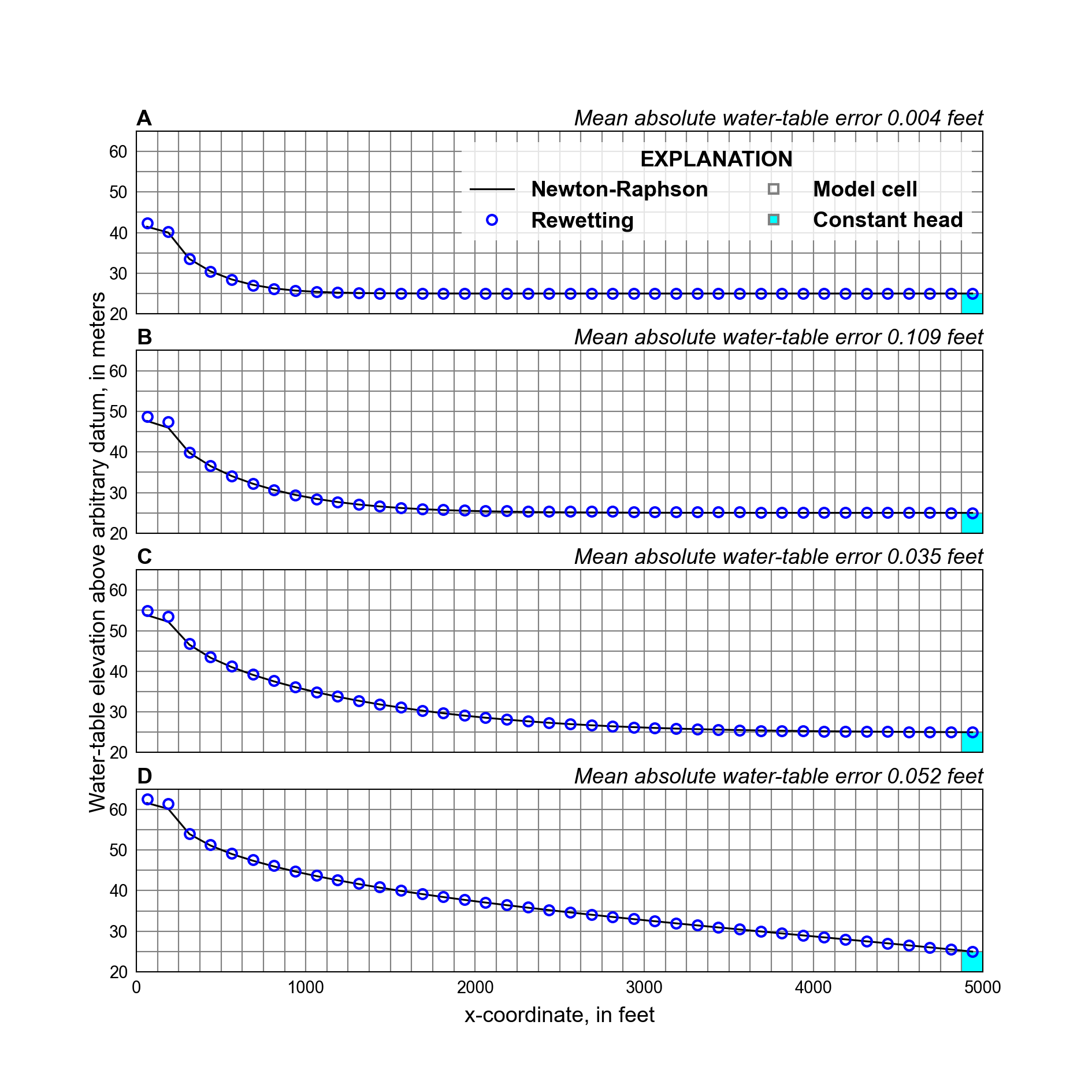
Figure 8.2 Comparison of water-table elevations simulated using the Newton-Raphson Formulation and Standard Conductance Formulation with rewetting. Water-table altitudes in row 1 are shown for A, 190 days, B, 708 days, C, 2,630 days, and D, at steady state. The location of the uppermost constant head boundary cell is also shown.
8.3. References Cited
Hughes, J. D., Langevin, C. D., & Banta, E. R. (2017). Documentation for the MODFLOW 6 framework. https://doi.org/10.3133/tm6A57
McDonald, M. G., Harbaugh, A. W., Orr, B. R., & Ackerman, D. J. (1992). A method of converting no-flow cells to variable-head cells for the U.S. Geological Survey modular finite-difference ground-water flow model. Retrieved from https://pubs.er.usgs.gov/publication/ofr91536
Niswonger, R. G., Panday, S., & Ibaraki, M. (2011). MODFLOW-NWT, A Newton formulation for MODFLOW-2005. Retrieved from https://pubs.er.usgs.gov/publication/tm6A37
8.4. Jupyter Notebook
The Jupyter notebook used to create the MODFLOW 6 input files for this example and post-process the results is: