69. Forward Particle Tracking, Structured Grid, Steady-State Flow
This example demonstrates a MODFLOW 6 particle tracking (PRT) model by reproducing example problem 1 from the MODPATH 7 (D. W. Pollock, 2016) example problems document (D. Pollock, 2017). An equivalent MODPATH 7 model is constructed for comparison, though only PRT results are shown.
69.1. Example description
The example first runs a groundwater flow (GWF) model simulating steady-state flow on a structured grid. The flow system includes an upper and lower aquifer separated by a confining layer with lower conductivity. The grid has 3 layers, 21 rows, and 20 columns, with square cells 500 feet to a side. The system includes two boundary conditions: a well in layer 3, row 11, column 10, and a river in layer 1, column 20 (fig Figure 69.1). Model parameters for this example are summarized in Table 69.1.
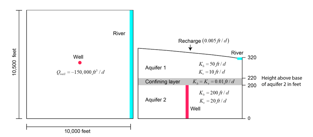
Figure 69.1 Conceptual model. Image reproduced from the MODPATH 7 examples document (D. Pollock, 2017).
Parameter |
Value |
|---|---|
Number of periods |
1 |
Number of layers |
3 |
Number of rows |
21 |
Number of columns |
20 |
Column width (\(ft\)) |
500.0 |
Row width (\(ft\)) |
500.0 |
Top of the model (\(ft\)) |
400.0 |
Layer bottom elevations (\(ft\)) |
220.0, 200.0, 0.0 |
Porosity (unitless) |
0.1 |
Recharge rate (\(ft/d\)) |
0.005 |
Horizontal hydraulic conductivity (\(ft/d\)) |
50.0, 0.01, 200.0 |
Vertical hydraulic conductivity (\(ft/d\)) |
10.0, 0.01, 20.0 |
Well pumping rate (\(ft^3/d\)) |
–150000.0 |
River stage (\(ft\)) |
320.0 |
River bottom (\(ft\)) |
317.0 |
River conductance (\(ft^2/d\)) |
1.0e5 |
69.2. Example Results
In this example a MODFLOW 6 particle tracking (PRT) model runs in the same simulation as a groundwater flow (GWF) model (fig Figure 69.2), which provides it with intercell flows via a GWF-PRT model exchange.

Figure 69.2 Heads simulated by the MODFLOW 6 groundwater flow (GWF) model.
In subproblem 1A, a line of 21 particles is placed at the water table in layer 1 for column 3, rows 1 through 21. In subproblem 1B, a denser release configuration is used which places a 3 x 3 array of particles on the top face of every cell in layer 1. Both simulations track particles forward to their discharge points.
Subproblem 1A path points on a 1000-day time interval are shown in fig Figure 69.3.

Figure 69.3 Particle pathlines and 1000-day points for subproblem 1A. Points are colored by layer.
To illustrate discharge points, pathlines are colored by discharge area (well or river) in fig Figure 69.4. To show capture areas, starting locations of all particles are color-coded according to the zone value of the cells in which they terminate in fig Figure 69.5. Travel time analysis is also a common use case for particle tracking. Particle release points are colored by total travel time to capture in fig Figure 69.6.

Figure 69.4 Particle pathlines, colored by destination: particles with red pathlines are captured by the well, particles with blue pathlines are captured by the river.

Figure 69.5 Particle release points, colored by destination.

Figure 69.6 Particle release points, colored by travel time.
69.3. References Cited
Pollock, D. (2017). MODPATH version 7: Example problems.
Pollock, D. W. (2016). User guide for MODPATH Version 7—A particle-tracking model for MODFLOW. https://doi.org/10.3133/ofr20161086
69.4. Jupyter Notebook
The Jupyter notebook used to create the MODFLOW 6 input files for this example and post-process the results is: