50. MT3DMS Supplemental Guide Problem 8.2
This example is for a recirculating well. It is based on example problem 8.2 described in (Zheng, 2010). The problem consists of a two-dimensional, one-layer model with flow from left to right. A solute is introduced into the flow field by an injection well. Downgradient, an extraction well pumps at the same rate as the injection well. This extracted water is then injected into two other injection wells. This example is simulated with the GWT Model in MODFLOW 6, which receives flow information from a separate simulation with the GWF Model in MODFLOW 6. Results from the GWT Model are compared with the results from a MT3DMS simulation (Zheng, 1990) that uses flows from a separate MODFLOW-2005 simulation (Harbaugh, 2005).
50.1. Example description
The parameters used for this problem are listed in Table 50.1. The model grid consists of 31 rows, 46 columns, and 1 layer. The flow problem is confined and steady state. The solute transport simulation represents transient conditions, which begin with an initial concentration specified as zero everywhere within the model domain.
For the MT3DMS representation of this problem, the Well Package is used to inject water at a rate of 1 \(m^3/d\) into model cell (1, 16, 16). Water is extracted at a rate of -1 \(m^3/d\) from model cell (1, 16, 21). Two additional wells, located in cells (1, 5, 16) and (1, 27, 16), reinject water at the concentration of the extracted water from cell (1, 16, 21). The injection rate for each of these reinjection wells is 0.5 \(m^3/d\).
For the MODFLOW 6 representation of this problem, the Multi-Aquifer Well (MAW) Package is used for these injection and extraction wells, although because the model is only a single layer, the MAW Package behaves just like the Well Package. The Water Mover (MVR) Package is used to send half of the extracted water into each of the reinjection wells. For the MODFLOW 6 transport simulation, the Multi-Aquifer Transport (MWT) Package is used to calculate the concentration in each of the well bores. The Mover Transport (MVT) Package is used to move the solute from the extraction well to the two reinjection wells based on the simulated flows. Note that this approach used in MODFLOW 6 is slightly different than the approach used in MT3DMS, because MODFLOW 6 is calculating the concentrations in the well boreholes rather than using concentrations directly from the model cells. By specifying a small well radius for the MAW Package, the approaches are similar.
Parameter |
Value |
|---|---|
Number of periods |
1 |
Number of layers |
1 |
Number of rows |
31 |
Number of columns |
46 |
Column width (\(m\)) |
10.0 |
Row width (\(m\)) |
10.0 |
Top of the model (\(m\)) |
10.0 |
Layer bottom elevation (\(m\)) |
0.0 |
Hydraulic conductivity (\(md^{-1}\)) |
10.0 |
Longitudinal dispersivity (\(m\)) |
10.0 |
Transverse horizontal dispersivity (\(m\)) |
3.0 |
Transverse vertical dispersivity (\(m\)) |
0.3 |
Simulation time (\(d\)) |
365.0 |
Porosity of mobile domain (unitless) |
0.3 |
50.2. Example Results
Simulated concentrations from MODFLOW 6 and MT3DMS are shown in Figure 50.1. The close agreement between the simulated concentrations demonstrate the ability of MODFLOW 6 to simulate the transfer of water and solute using the mover package capability.
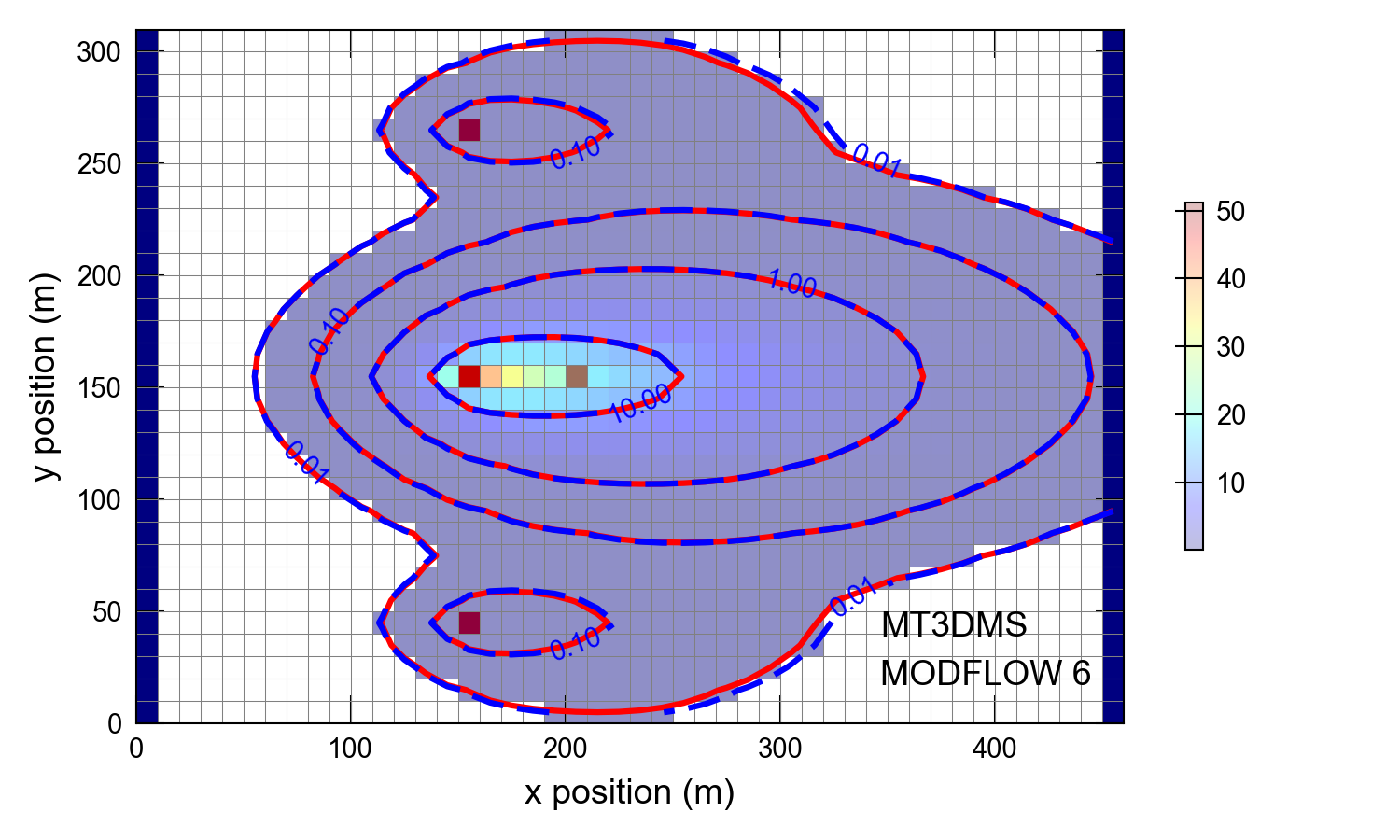
Figure 50.1 Concentrations simulated by MODFLOW 6 and MT3DMS for a problem involving a recirculating well. This figure can be compared to figure 8.2 in (Zheng, 2010).
50.3. References Cited
Harbaugh, A. W. (2005). MODFLOW-2005, the U.S. Geological Survey modular ground-water model—the Ground-Water Flow Process. Retrieved from https://pubs.usgs.gov/tm/2005/tm6A16/
Zheng, C. (1990). MT3D, a modular three-dimensional transport model for simulation of advection, dispersion and chemical reactions of contaminants in groundwater systems.
Zheng, C. (2010). MT3DMS v5.3—a modular three-dimensional multi-species transport model for simulation of advection, dispersion and chemical reactions of contaminants in groundwater systems; supplemental user’s guide.
50.4. Jupyter Notebook
The Jupyter notebook used to create the MODFLOW 6 input files for this example and post-process the results is: