39. MT3DMS Problem 3
This is the third problem appearing in (Zheng & Wang, 1999), titled, “two-dimensional transport in a uniform flow field.” In contrast to the first demonstrated examples, transport is simulated in two dimensions with dispersion but no reactions. An analytical solution for this problem was originally published in (Wilson & Miller, 1978). Two assumptions that make the analytical solution possible are that (1) the aquifer is areally infinite and relatively thin to support the assumption that instantaneous mixing occurs in the vertical direction, and (2) that compared to the ambient flow field, the injection rate is insignificant.
39.1. Example description
Steady uniform flow enters the left edge of a numerical grid with 31 rows, 46 columns, and 1 layer through a constant head boundary and exits along the right edge. Constant heads are selected to ensure the hydraulic gradient matches with the analytical solution. The other boundaries are all no flow. Boundaries are sufficiently far away from the injection well where the contaminant is released so as not to interfere with the final solution after 365 days. Table 39.1 summarizes model setup:
Parameter |
Value |
|---|---|
Number of layers |
1 |
Number of rows |
31 |
Number of columns |
46 |
Column width (\(m\)) |
10.0 |
Row width (\(m\)) |
10.0 |
Layer thickness (\(m\)) |
10.0 |
Top of the model (\(m\)) |
0.0 |
Porosity |
0.3 |
Simulation time (\(days\)) |
365 |
Horizontal hydraulic conductivity (\(m/d\)) |
1.0 |
Volumetric injection rate (\(m^3/d\)) |
1.0 |
Concentration of injected water (\(mg/L\)) |
1000.0 |
Longitudinal dispersivity (\(m\)) |
10.0 |
Ratio of transverse to longitudinal dispersivity |
0.3 |
After 365 days, the MODFLOW 6 solution aligns well with the MT3DMS solution (Figure 39.1). In addition to the good agreement that was seen in the first MT3DMS test problem, the current comparison confirms that the lateral dispersion is accurately simulated within MODFLOW 6.
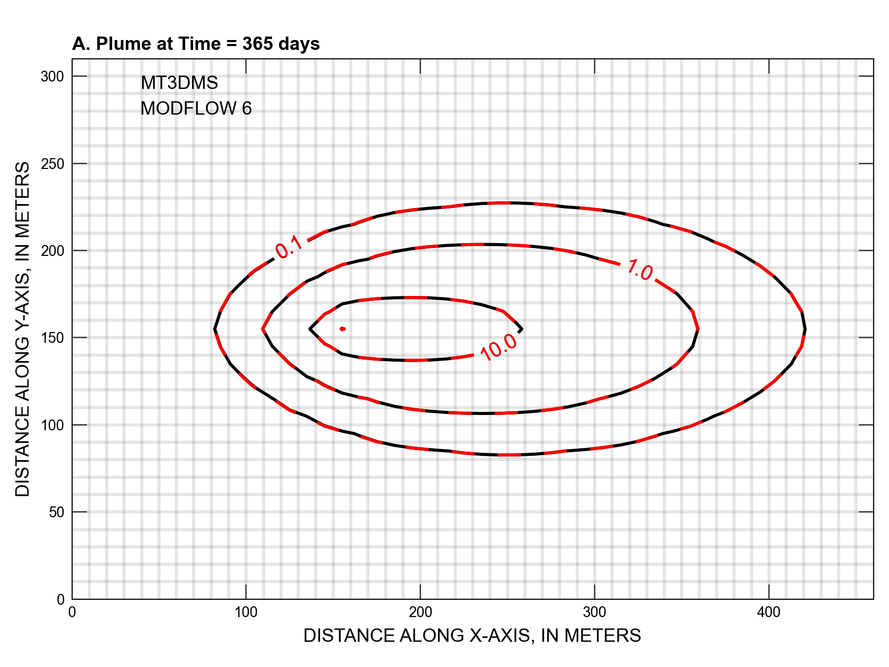
Figure 39.1 Comparison of the MT3DMS and MODFLOW 6 numerical solutions for a two-dimensional advection-dispersion test problem. The analytical solution for this problem was originally given in (Wilson & Miller, 1978) and is not shown here
39.2. References Cited
Wilson, J. L., & Miller, P. J. (1978). Two-dimensional plume in uniform ground-water flow. Journal of the Hydraulics Division, 104(4), 503–514. https://doi.org/10.1061/JYCEAJ.0004975
Zheng, C., & Wang, P. P. (1999). MT3DMS—a modular three-dimensional multi-species transport model for simulation of advection, dispersion and chemical reactions of contaminants in groundwater systems; documentation and user’s guide.
39.3. Jupyter Notebook
The Jupyter notebook used to create the MODFLOW 6 input files for this example and post-process the results is: