57. Radial Groundwater Flow Model
Radial groundwater models simulate and analyze the flow of groundwater in a radial coordinate system. The purpose of radial groundwater models is to understand the behavior of groundwater flow in response to groundwater extraction or to estimate aquifer properties. Radial groundwater models are axisymmetric with the constant aquifer properties defined in circular radial bands and vertical layers. The radial grid’s innermost band is cylinder (single radius) and typically contains a groundwater well. Extending outward, the subsequent radial bands are ring shaped that are bound by an inner and outer radius (hollow cylinder). This example demonstrates the capability of the Unstructured Discretization (DISU) Package to represent a radial groundwater flow model.
This example replicates in MODFLOW 6 using FloPy the “Pumping Well” radial model described in (Bedekar et al., 2019). The original model used MODFLOW-USG to demonstrate that it is possible to use unstructured grid cells to simulate a banded, radial model. The MODFLOW 6 results are compared with the (Neuman, 1974) analytical solution for radial, unconfined flow with a partially penetrating well.
57.1. Example description
The example consists of a multi-layer, radial model representing an unconfined, homogeneous, and isotropic aquifer with a partially penetrating well. The radial grid represents the horizontal direction and is composed of 22 radial bands that vary in outer radius from 0.25 \(ft\) to 2000 \(ft\) (Figure 57.1A). Radial band 1 is a cylinder with a radius 0.25 \(ft\) and radial band 22 is a hollow cylinder with an inner and outer radius of 1500 \(ft\) and 2000 \(ft\), respectively. The vertical direction consists of 25 uniform-layers that are 2 \(ft\) thick; with a total aquifer thickness of 50 \(ft\). A partially penetrating well is located at radial band 1 (Figure 57.1B) and extracts water from the bottom 10 \(ft\) (layer 21 to 25) at a rate of 4000 \(ft^3/day\). The remaining model properties are summarized in Table 57.1.
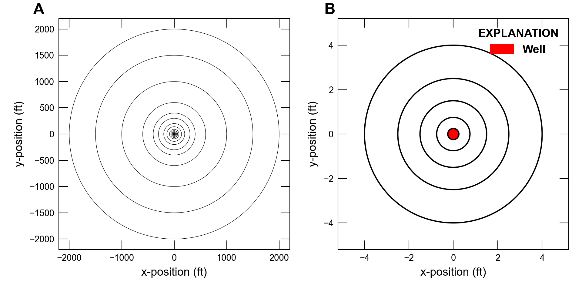
Figure 57.1 Plan view of the two-dimensional, radial model grid. A, plan view of entire model grid containing 22 radial bands, and B, plan view of the 5 innermost radial bands and the well location is marked in red.
The model simulation evaluates drawdown in response to pumping at an observation point. The simulation time frame is composed of 1 stress period of length 10 \(days\), subdivided into 24 time steps with a multiplier of 1.24. The aquifer is initially saturated with an initial water level is set to 50 \(ft\), which is the reference level for drawdown. Observations are made at a radial distance of 40 \(ft\) (radial band 12) at the model’s top (1 \(ft\) depth; layer 1), middle (25 \(ft\) depth; layer 13), and bottom (49 \(ft\) depth; layer 25) for every time step.
Parameter |
Value |
|---|---|
Number of periods |
1 |
Number of time steps |
24 |
Simulation total time (\(day\)) |
10 |
Number of layers |
25 |
Number of radial direction cells (radial bands) |
22 |
Initial water table elevation (\(ft\)) |
50.0 |
Top of the radial model (\(ft\)) |
50.0 |
Base of the radial model (\(ft\)) |
0.0 |
Thickness of each radial layer (\(ft\)) |
2.0 |
Outer radius of each radial band (\(ft\)) |
0.25 to 2000 |
Horizontal hydraulic conductivity (\(ft/day\)) |
20.0 |
Vertical hydraulic conductivity (\(ft/day\)) |
20.0 |
Specific storage (\(1/day\)) |
1.0e-5 |
Specific yield (unitless) |
0.1 |
Well screen elevation (\(ft\)) |
0.0 to 10 |
Well radial band location (unitless) |
1 |
Well pumping rate (\(ft^3/day\)) |
–4000.0 |
Observation distance from well (\(ft\)) |
40 |
“Top” observation elevation (\(ft\)) |
1 |
“Middle” observation depth (\(ft\)) |
25 |
“Bottom” observation depth (\(ft\)) |
49 |
57.2. Radial Setup with Unstructured Discretization (DISU)
To represent a radial grid, the DISU defines cell connectivity based on radial band circumference, circular areas, and the radial distance between bands. All radial bands have the same properties for each layer. That is, each layer’s radial band has the same radius, circumference and area and only shifts the top and bottom elevation downward by 2 \(ft\). A maximum of 4 connections is possible for any given node; the connections represent flow towards the inner band, to the outer band, upward flow, and downward flow.
Node numbers are assigned based on the radial band number (R), layer number (L), and the total number of radial bands (nradial) as described in equation 57.1.
To make the following more compact, radial band and layer numbers are presented as “(R, L)” pairs. The first node is (1, 1) and is a cylinder that is connected to the next radial band, (2, 1), and the cylinder beneath it, (1, 2). The nodal connections (JA) for node 1 is then nodes 2 and 23. The second node, (2, 1), is connected to the inner band at (1, 1), an outer band at (3, 1), and the downward band (2, 2). The JA connections for node 2 is then nodes 1, 3, and 24. Similarly node 24 is located at (2, 2) is connected to the inner band (1, 2), outer band (3, 2), upward band (2, 1), and downward band (2, 3). The JA connections for node 24 is then nodes 23, 25, 2, and 46, respectively.
The input requires specifying the plan view, cell surface area. This is calculated using equation 57.2.
where \(r\) is the outer radius for radial band \(j\) and \(r_0=0\). The surface area for any radial band is the same for all layers.
The connection length (CL12) depends on if the cell connection is in the vertical or radial direction. Vertical connections are half the distance between the top and bottom elevation of the cell. Since all cells have a thickness of 2 \(ft\), CL12 is 1 \(ft\) for all vertical connections. The radial direction has a CL12 for radial band 1 equal to its outer radius. For the rest of the radial bands CL12 is same for both the inner and outer directions and is half the distance between the inner and outer radius. That is, \(\text{CL12}_j = 0.5\left(r_j-r_{j-1}\right)\), where \(r\) is the outer radius for radial band \(j\) and \(r_0={-r}_1\).
The input HWVA is the plan view area (\(ft^2\)) for vertical connections and the width (\(ft\)) perpendicular to flow for horizontal connections. Since all layers have the same radii, the vertical \(\text{HWVA}_j\) is equal to \(\text{AREA}_j\). The horizontal HWVA width is equal the radial band’s circumference (\(2\pi r\)) that the flow passes through. For flow towards the inner band, \(\text{HWVA}_{j,\ \text{inner}} = 2\pi r_{j-1}\), and towards the outer band, \(\text{HWVA}_{j,\ \text{outer}}\ = 2\pi r_j\).
To assist with the FloPy setup a script called get_disu_radial_kwargs.py
is provided. This script provides the function
get_disu_radial_kwargs that assembles the nodal connections and
aforementioned properties (JA, AREA, CL12, HWVA). The function input
expects the number of layers, number of radial bands, outer radius for
each band, surface elevations, and layer thicknesses.
57.3. Example Results
Figures Figure 57.2 and Figure 57.3 present the simulated head and dimensionless drawdown results of the radial model with an initial head of 50 \(ft\) and 4000 \(ft^3/d\) pumping for 10 days. In the figures the circles represent the MODFLOW 6 (MF6) solution at the end of the time step and the lines are the analytical solution from Equation 17 in (Neuman, 1974). The analytical solution uses dimensionless time and drawdown, so the results are presented in both head (MF6 native solution; Figure 57.2) and dimensionless drawdown (analytical native solution; Figure 57.3). Dimensionless time with respect to specific yield and dimensionless drawdown are defined as:
where \(t_y\) is dimensionless time with respect to specific yield (-), \(T\) is the initial, radial direction transmissivity (\(ft^2/d\)), \(t\) is the simulation time (\(d\)), \(S_y\) is the specific yield (-), \(r\) is the radial distance from the well to the observation point (\(ft\)), \(s_d\) is dimensionless drawdown (-), \(s\) is the drawdown from the initial water table elevation (\(ft\)), and \(Q\) is the pumping rate (\(ft^3/d\)).
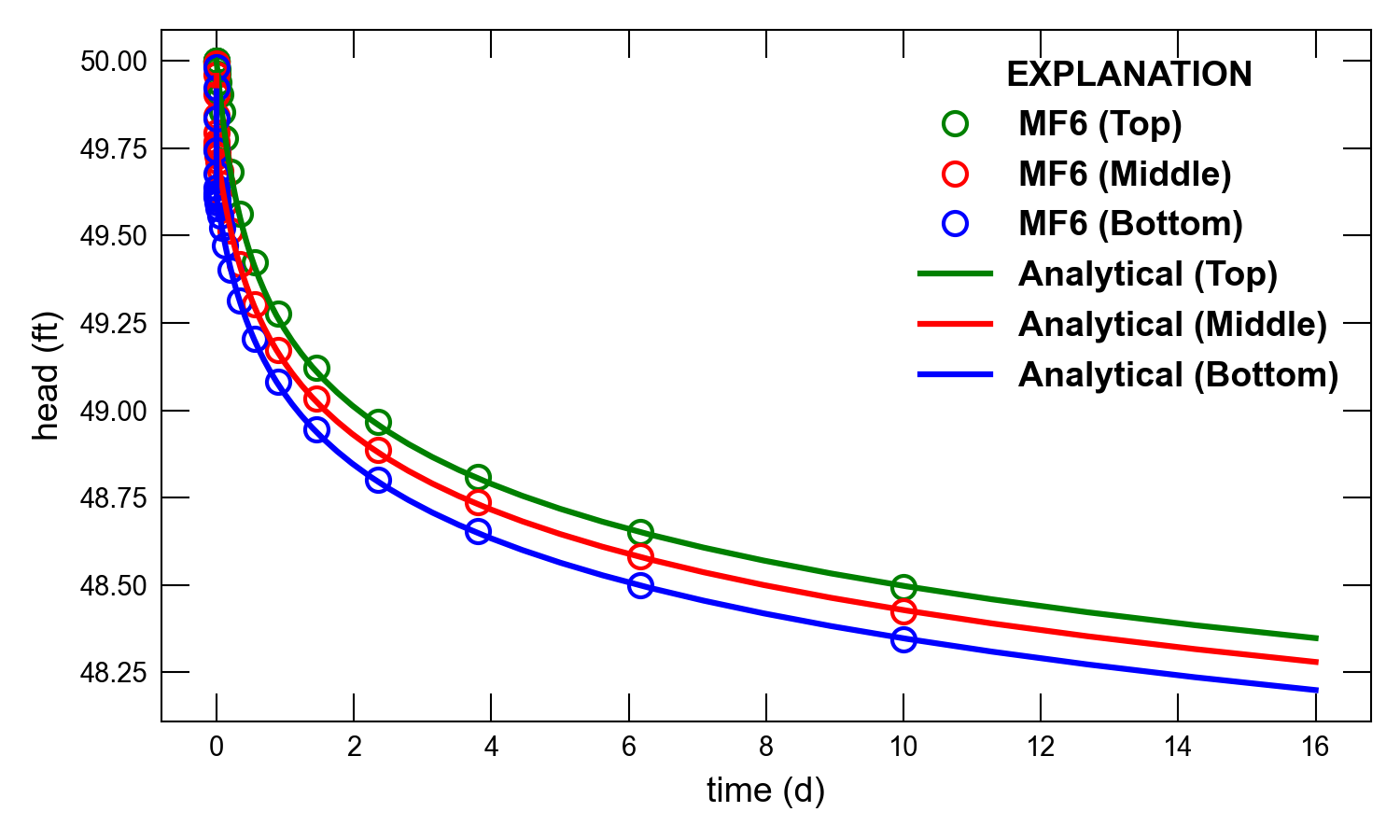
Figure 57.2 Radial model analytical solution (Neuman, 1974) and simulated groundwater (MF6) head 40 \(ft\) from the well (radial band 12) at the model’s Top (1 \(ft\) depth; layer 1), Middle (25 \(ft\) depth; layer 13), and Bottom (49 \(ft\) depth; layer 25).
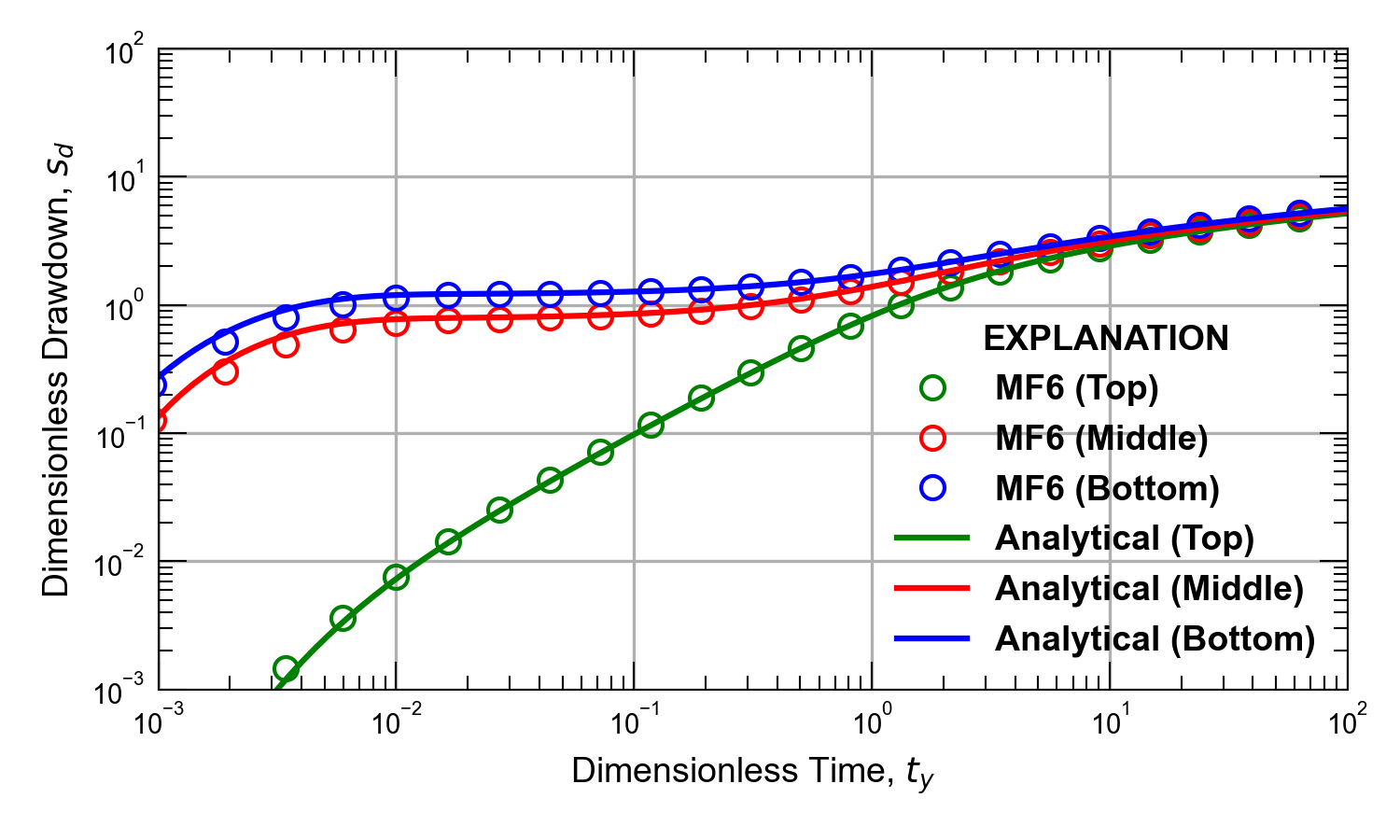
Figure 57.3 Radial model analytical dimensionless solution (Neuman, 1974) and simulated groundwater (MF6) dimensionless drawdown 40 \(ft\) from the well (radial band 12) at the model’s Top (1 \(ft\) depth; layer 1), Middle (25 \(ft\) depth; layer 13), and Bottom (49 \(ft\) depth; layer 25).
In Figure 57.2, the MF6 head compare very well to the analytical solution. In Figure 57.3, the MF6 dimensionless drawdown deviates from the analytical solution initially and then yields similar results. This deviation is more apparent in the first four circles (from the left) because of the small numbers presented on a log-log plot. These errors occur in the first 50 seconds of the 10-day simulation and are negligible in comparison to the rest of the simulation.
57.4. References Cited
Bedekar, V., Scantlebury, L., & Panday, S. (2019). Axisymmetric modeling using MODFLOW-USG. Groundwater, 57(5), 772–777. https://doi.org/10.1111/gwat.12861
Neuman, S. P. (1974). Effect of partial penetration on flow in unconfined aquifers considering delayed gravity response. Water Resources Research, 10(2), 303–312. https://doi.org/10.1029/WR010i002p00303
57.5. Jupyter Notebook
The Jupyter notebook used to create the MODFLOW 6 input files for this example and post-process the results is: