42. MT3DMS Problem 6
In this example problem, concentrations are compared between MODFLOW 6 and MT3D-USGS at an injection/extraction well. The well is fully penetrating in a confined aquifer and injects contaminated water for a period of 2.5 years at a rate of 1 \(ft^3/sec\). At the end of 2.5 years, the injection well is reversed and begins pumping (extracting) contaminated groundwater for a period of 7.5 years, also at the rate of 1 \(ft^3/sec\). (El‐Kadi, 1988) was the first to develop the test problem which was later used by (Zheng, 1993) to test ongoing method-of-characteristics (MOC) developments. The model boundary is placed far enough away from the injection/extraction well to ensure no solute exits the model domain during the injection period. Moreover, steady flow conditions are reached immediately during the injection and extraction stress periods. Problem specifics are provided in Table 42.1.
Parameter |
Value |
|---|---|
Number of layers |
1 |
Number of rows |
31 |
Number of columns |
31 |
Column width (\(ft\)) |
900.0 |
Row width (\(ft\)) |
900.0 |
Layer thickness (\(ft\)) |
20.0 |
Top of the model (\(ft\)) |
0.0 |
Porosity |
0.35 |
Length of the injection period (\(years\)) |
2.5 |
Length of the extraction period (\(years\)) |
7.5 |
Horizontal hydraulic conductivity (\(ft/d\)) |
432.0 |
Volumetric injection rate (\(ft^3/d\)) |
1.0 |
Relative concentration of injected water (\(\%\)) |
100.0 |
Longitudinal dispersivity (\(ft\)) |
100.0 |
Ratio of transverse to longitudinal dispersitivity |
1.0 |
An analytical solution for this problem was originally given in (Gelhar & Collins, 1971). Because this is an advection dominated problem, both numerical solutions invoke their TVD schemes. The MODFLOW 6 solution shows a quicker rise in concentration at the well site than does the MT3D-USGS solution (Figure 42.1).
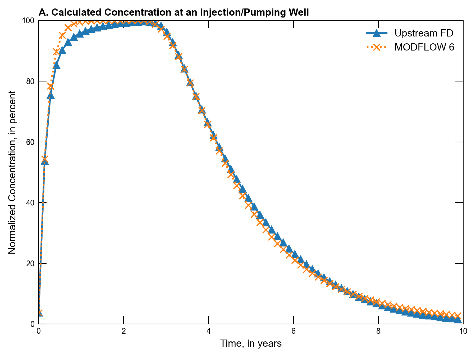
Figure 42.1 Comparison of the MT3D-USGS and MODFLOW 6 numerical solutions at an injection/extraction well. The analytical solution for this problem was originally given in (Gelhar & Collins, 1971) and is not shown here
42.1. References Cited
El‐Kadi, A. L. (1988). Applying the USGS mass‐transport model (MOC) to remedial actions by recovery wells. Groundwater, 26(3), 281–288. https://doi.org/10.1111/j.1745-6584.1988.tb00391.x
Gelhar, L. W., & Collins, M. A. (1971). General analysis of longitudinal dispersion in nonuniform flow. Water Resources Research, 7(6), 1511–1521. https://doi.org/0.1029/WR007i006p01511
Zheng, C. (1993). Extension of the method of characteristics for simulation of solute transport in three dimensions. Groundwater, 31(3), 456–465. https://doi.org/10.1111/j.1745-6584.1993.tb01848.x
42.2. Jupyter Notebook
The Jupyter notebook used to create the MODFLOW 6 input files for this example and post-process the results is: