45. MT3DMS Problem 9
This example compares MODFLOW 6 and MT3DMS transport solutions in a two-dimensional plan-view setting with heterogeneity in the hydraulic conductivity field. The problem is purely hypothetical and was originally used for comparing different MT3DMS solutions (i.e., finite-difference, method-of-characteristics, and TVD advection schemes) to each other. No analytical solution exists for this problem (Zheng & Wang, 1999).
45.1. Example description
A contaminant plume originates in an injection well located near the upper portion of the model (Figure 45.1). After its injection, contaminant migrates toward a pumping well located several rows below a low hydraulic conductivity zone, itself located a couple rows below where contaminant enters the aquifer.
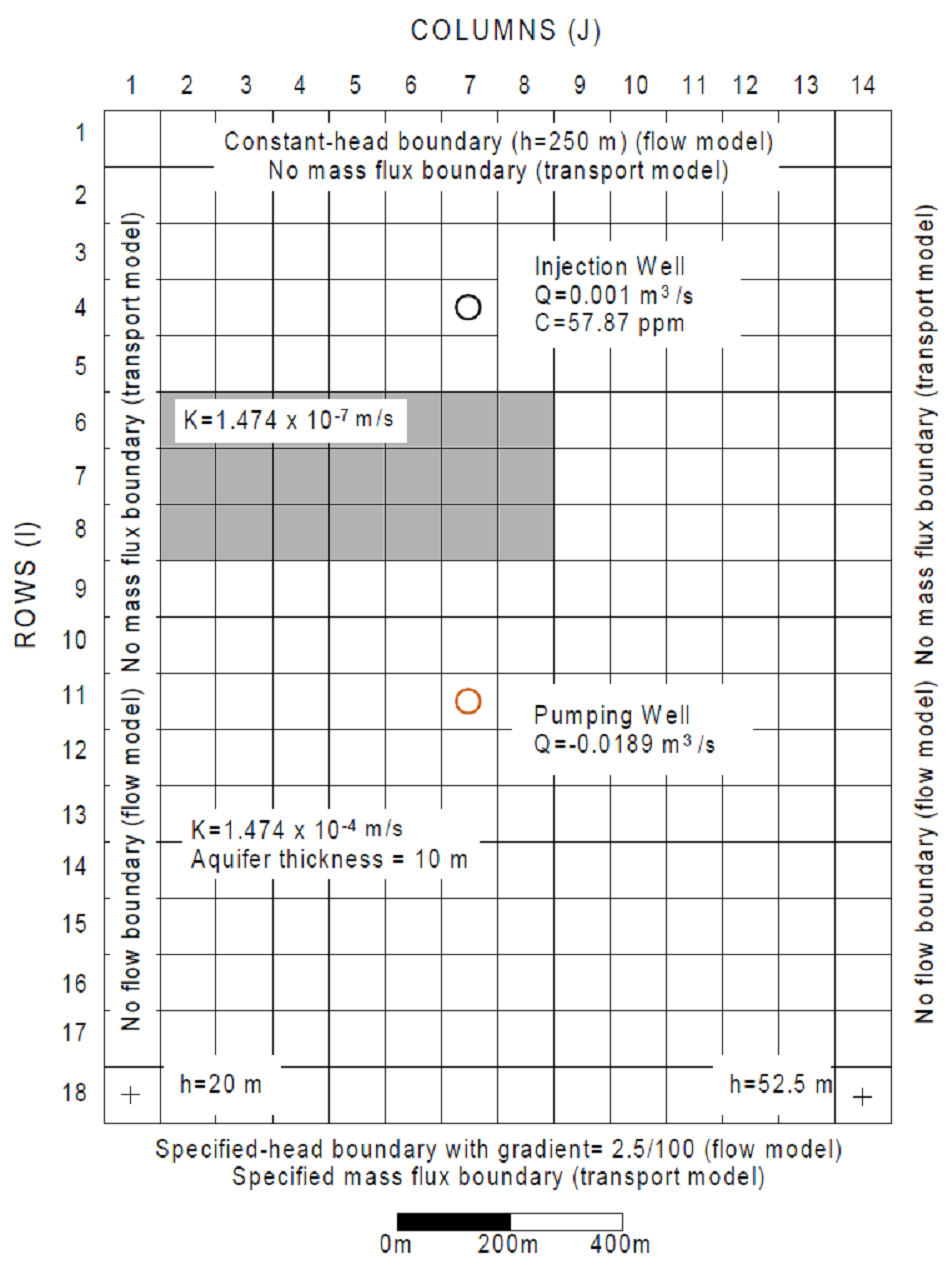
Figure 45.1 MT3DMS test problem 9 configuration showing grid discretization, constant head boundaries, and the locations of injection and pumping wells (from (Zheng & Wang, 1999)).
The model domain is discretized by 18 rows, 14 columns, and a single confined layer. Grid cell dimensions are uniformly set to 100 \(\times\) 100 \(m\). The left, right and bottom model boundaries are noo-flow. The upper (north) boundary applies a specified head of 250 \(m\) that is held constant throughout the simulation period. Similarly, a specified head is applied to the lower (south) boundary that varies from 20 \(m\) on the left to 52.5 \(m\) on the right, a gradient of 2.5/100 \(m/m\). Water injected into the aquifer enters at a concentration of 57.87 \(ppm\). Mass is removed from the aquifer by both the pumping well and with the flow that exits the domain at the lower (south) boundary of the model. Mass that exits the lower boundary does so at the simulated concentration of the water that is removed by the constant head boundary condition. Mass is not allowed to leave through the upper, bottom, left, or right boundaries in the respective transport simulations. All flow boundary conditions are held constant for the duration of the simulation period, resulting in steady-flow conditions. However, the concentration of the injected water is reduced to 0.0 \(ppm\) during the second of two stress periods. Both the injection and pumping wells are assumed to be fully penetrating. Aquifer heterogeneity is depicted in Figure 45.1. Model parameters are summaried in Table 45.1.
Parameter |
Value |
|---|---|
Number of layers |
1 |
Number of rows |
18 |
Number of columns |
14 |
Column width (\(m\)) |
100.0 |
Row width (\(m\)) |
100.0 |
Layer thickness (\(m\)) |
10.0 |
Top of the model (\(m\)) |
0.0 |
Porosity |
0.3 |
Horiz. hyd. conductivity of fine grain material (\(m/sec\)) |
1.474e-4 |
Horiz. hyd. conductivity of medium grain material (\(m/sec\)) |
1.474e-7 |
Injection well rate (\(m^3/sec\)) |
0.001 |
Extraction well pumping rate (\(m^3/sec\)) |
–0.0189 |
Longitudinal dispersivity (\(m\)) |
20.0 |
Ratio of horiz. transverse to longitudinal dispersivity (\(m\)) |
0.2 |
Simulation time (\(years\)) |
2.0 |
In MODFLOW 6, the XT3D solver is not activated; however, both MODFLOW 6 and MT3DMS use their respective TVD advection schemes.
45.2. Example results
Contrasting model results after one year, the leading edge of the plume advanced further within the MODFLOW 6 solution (Figure 45.2). Confirmation that the same amount of mass entered both simultions (MODFLOW 6 and MT3DMS) was achieved by checking the mass budget information in the respective mode output listing files. In both simulations, the effect of the aquitard aquitard is clearly seen, though the isoconcentration lines appear to have infiltrated the aquitard more with MT3DMS compared to the MODFLOW 6 solution.
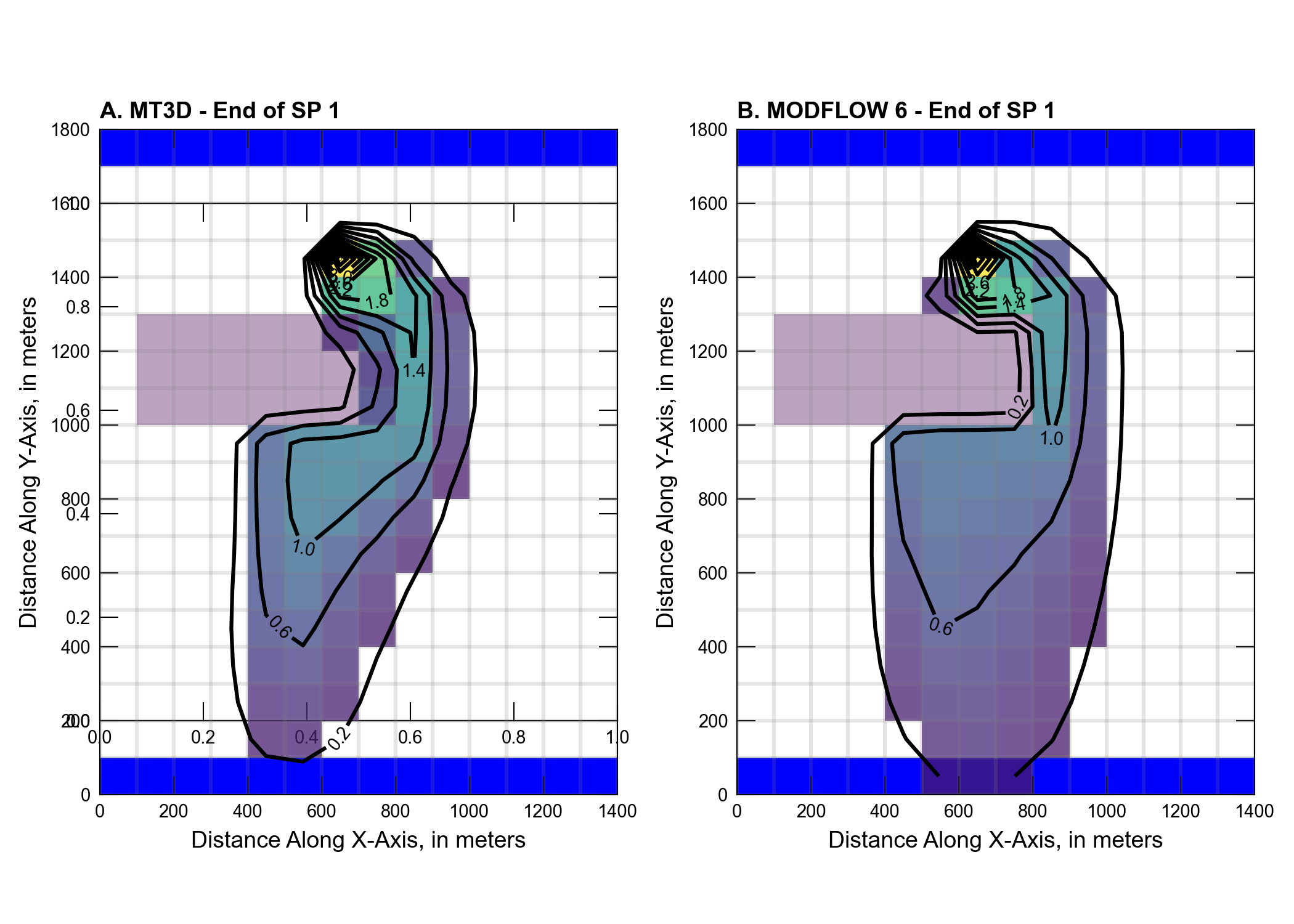
Figure 45.2 Migrating contaminant plume as calculated by (A) MT3D-USGS and (B) MODFLOW 6 after one year of simulation time. The original problem was given in (Zheng & Wang, 1999). Cells shaded in blue show the location of constant head boundary cells. Light brown shaded cells show the location of the aquitard.
45.3. References Cited
Zheng, C., & Wang, P. P. (1999). MT3DMS—a modular three-dimensional multi-species transport model for simulation of advection, dispersion and chemical reactions of contaminants in groundwater systems; documentation and user’s guide.
45.4. Jupyter Notebook
The Jupyter notebook used to create the MODFLOW 6 input files for this example and post-process the results is: