2. BCF2SS Model
In an aquifer system where two aquifers are separated by a confining bed, large pumpage withdrawals from the bottom aquifer can desaturate parts of the upper aquifer. If pumpage is discontinued, resaturation of the upper aquifer can occur. This problem demonstrates the capability of the Node Property Flow (NPF) Package to successfully simulate this common hydrologic situation which is difficult or impossible to simulate without use of the rewetting option and the Standard Formulation or the Newton-Raphson Formulation.
This example is a version of the original MODFLOW rewetting example (BCF2SS) described in (McDonald et al., 1992). This problem is also is distributed with MODFLOW-2005 (Harbaugh, 2005). The problem has been modified to use a vertical hydraulic conductivity that is equivalent to the original quasi-3D vertical conductance (VCONT) value used in the original problem.
2.1. Conceptual Model
The hypothetical aquifer system consists of a upper aquifer and a lower aquifer separated by a confining unit. No-flow boundaries surround the system on all sides, except that the lower aquifer discharges to a stream along the right side of the area (Figure 2.1). Recharge from precipitation is applied evenly over the entire area. The stream penetrates the lower aquifer; in the region above the stream, the upper aquifer and confining unit are missing (see McDonald et al., 1992, fig. 1). Under natural conditions, recharge flows through the system to the stream. Under stressed conditions, two wells withdraw water from the lower aquifer. If enough water is pumped, cells in the upper aquifer will desaturate. Removal of the stresses will then cause the desaturated areas to resaturate.
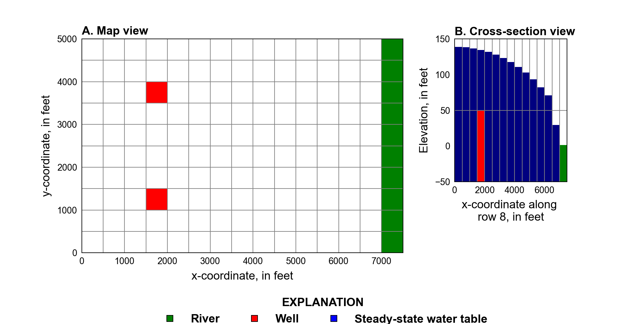
Figure 2.1 Diagram showing the model domain. A, plan view, and B, cross-section view. The locations of river cells, and wells are also shown. The steady-state water-table is shown in the cross-section view.
2.2. Example Description
The model consists of two layers–one for each aquifer. A uniform horizontal grid of 10 rows and 15 columns is used (Figure 2.1). Two steady-state solutions were obtained to simulate natural conditions and pumping conditions.
Because horizontal flow in the confining bed is small compared to horizontal flow in the aquifers and storage is not a factor in steady-state simulations, the confining bed is not treated as a separate layer. A horizontal hydraulic conductivity of 10 and 5 \(ft/day\) is specified for the upper and lower aquifers, respectively (Table 1.1); the horizontal conductivity of the lower aquifer is calculated based on the transmissivity (500 \(ft^2/day\)) and 100 \(ft\) layer thickness used in the original problem (McDonald et al., 1992). The vertical hydraulic conductivity of the confining units is calculated from the vertical conductance of the confining beds defined in the original problem (\(0.9999999 \times 10^{-3}\) per day) (Table 1.1).
Parameter |
Value |
|---|---|
Number of periods |
2 |
Number of layers |
2 |
Number of rows |
10 |
Number of columns |
15 |
Column width (\(ft\)) |
500.0 |
Row width (\(ft\)) |
500.0 |
Top of the model (\(ft\)) |
150.0 |
Layer bottom elevations (\(ft\)) |
50.0, –50. |
Cell conversion type |
1, 0 |
Horizontal hydraulic conductivity (\(ft/d\)) |
10.0, 5.0 |
Vertical hydraulic conductivity (\(ft/d\)) |
0.1 |
Starting head (\(ft\)) |
0.0 |
Recharge rate (\(ft/d\)) |
0.004 |
An initial head of zero \(ft\) is specified in all model layers. Flow into the system is from infiltration from precipitation and was represented using the recharge (RCH) package. A constant recharge rate of \(4 \times 10^{-3}\) \(ft/day\) was specified for every cell in the upper aquifer. Flow out of the model is from a stream represented by river (RIV) package cells in the lower aquifer, discharging wells represented by well (WEL) package cells in the lower aquifer. River cells are located in column 15 of every row in the lower aquifer and have a river stage, conductance, and bottom elevation of 0 \(ft\), 10,000 \(ft^2/day\), and -5 \(ft\), respectively (Figure 2.1). Two wells are included in the second stress period, each pumping 35,000 \(ft^3/day\), at (row 3, column 4) and (row 8, column 4) in the lower aquifer.
The WETDRY parameter used in upper aquifer is shown in Figure 2.2. On the right side of the model, the WETDRY parameter is negative in order to cause a cell to become wet only when head in the layer below exceeds the wetting threshold. This was done to avoid incorrectly converting dry cells to wet because of the large head differences between adjacent horizontal cells (McDonald et al., 1992). On the left side of the model, horizontal head changes between adjacent cells generally are small, so head in the neighboring horizontal cells is a good indicator of whether or not a dry cell should become wet. Therefore, positive WETDRY parameters are used in most of this area to allow wetting to occur either from the cell below or from horizontally adjacent cells. Near the well, the horizontal head gradients under pumping conditions also are relatively large; consequently, a negative WETDRY parameter was used at the cells above the well. This prevents these cells from incorrectly becoming wet (McDonald et al., 1992). Rewetting is not enabled in the lower aquifer.
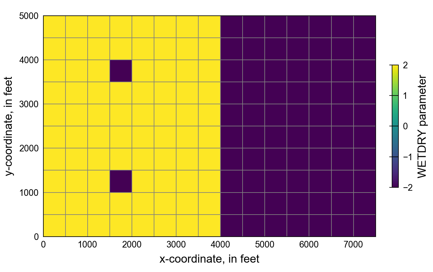
Figure 2.2 WETDRY parameter values used in the upper aquifer. Cells with negative values can only rewet when the head in an underlying cells exceeds the bottom of the cell. Cells with positive values can rewet if the head in an underlying cells exceeds the bottom of the cell or from adjacent connected cells.
2.3. Example Results
Two steady-state solutions were obtained to simulate natural conditions and pumping conditions. The two solutions are designed to demonstrate the ability of the rewetting option of the NPF Package to handle a broad range of possibilities for cells converting between wet and dry in the top aquifer. When solving for natural conditions, the top aquifer initially is specified as being entirely dry and many cells must convert to wet. When solving for pumping conditions, the top aquifer is initially specified to be under natural conditions and many cells must convert to dry. The first stress period simulates natural conditions (Figure 2.3A and B) and the second period simulates the addition of pumping wells (Figure 2.3C and D) .
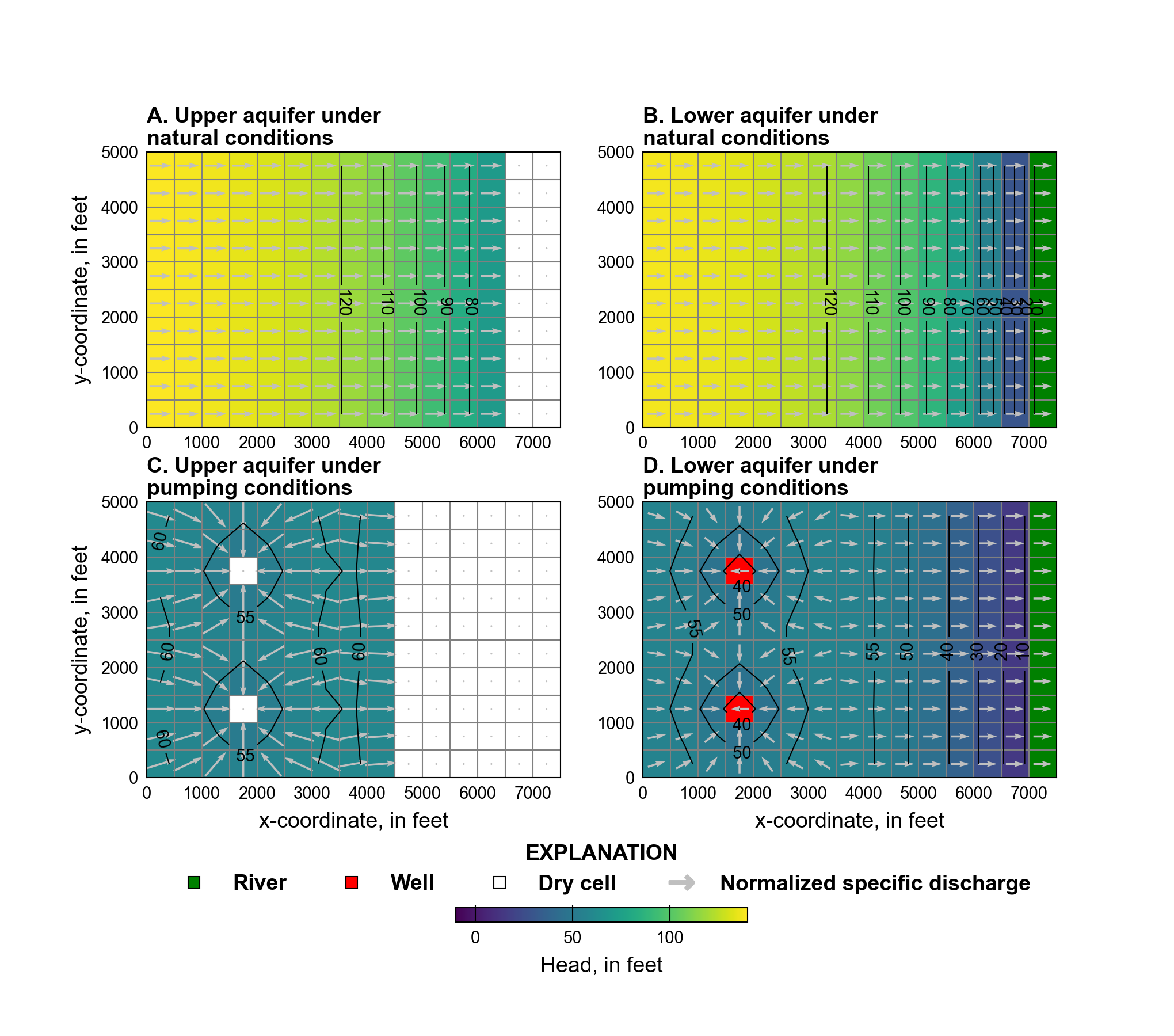
Figure 2.3 Simulated water levels and normalized specific discharge vectors in the upper and lower aquifers under natural and pumping conditions using the rewetting option in the Node Property Flow (NPF) Package with the Standard Conductance Formulation. A. Upper aquifer results under natural conditions. B. Lower aquifer results under natural conditions C. Upper aquifer results under pumping conditions. D. Lower aquifer results under pumping conditions
Simulated results for the example problem using the Newton-Raphson Formulation instead of the rewetting option and the Standard Formulation is shown in Figure 2.4. In general, the simulated results are comparable for the Standard Formulation with the NPF Package rewetting option and the Newton-Raphson formulation. The largest differences between the two approaches occur in the upper aquifer under pumping conditions and is the result of differences in horizontal conductance weighting. Upstream weighting, which is used with the Newton-Raphson Formulation, increases the volumetric horizontal flow and decreases water-levels. Also note how saturated conditions propagate further into the domain in the upper aquifer under pumping conditions using the Newton-Raphson Formulation than when the Standard Formulation with the NPF Package rewetting option is used.
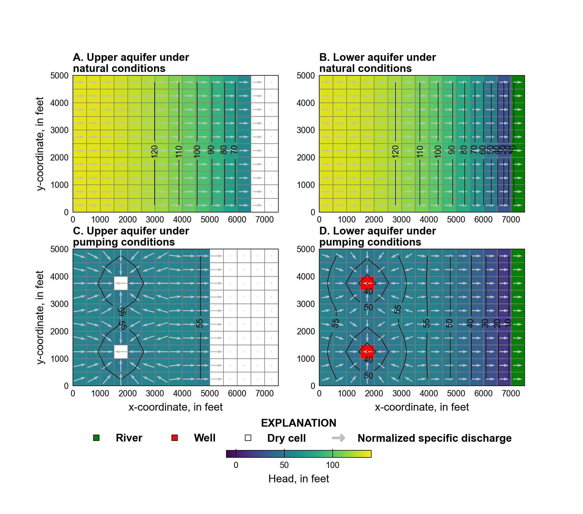
Figure 2.4 Simulated water levels and normalized specific discharge vectors in the upper and lower aquifers under natural and pumping conditions using the Newton-Raphson Formulation. A. Upper aquifer results under natural conditions. B. Lower aquifer results under natural conditions C. Upper aquifer results under pumping conditions. D. Lower aquifer results under pumping conditions
2.4. References Cited
Harbaugh, A. W. (2005). MODFLOW-2005, the U.S. Geological Survey modular ground-water model—the Ground-Water Flow Process. Retrieved from https://pubs.usgs.gov/tm/2005/tm6A16/
McDonald, M. G., Harbaugh, A. W., Orr, B. R., & Ackerman, D. J. (1992). A method of converting no-flow cells to variable-head cells for the U.S. Geological Survey modular finite-difference ground-water flow model. Retrieved from https://pubs.er.usgs.gov/publication/ofr91536
2.5. Jupyter Notebook
The Jupyter notebook used to create the MODFLOW 6 input files for this example and post-process the results is: