21. Hani Problem
This problem simulates groundwater flow to a pumping well under horizontally anisotropic groundwater flow conditions. This is a synthetic example problem that has not been documented elsewhere.
21.1. Example Description
Model parameters for the example are summarized in Table 21.1. The model consists of a grid of 51 columns, 51 rows, and 1 layer. The discretization is 10 \(m\) in the row and column direction for all cells (Figure 21.1). The top of the aquifer is zero and the bottom elevation of the aquifer is -10 \(m\). A single steady-stress period with a total length of 1 day is simulated.
Parameter |
Value |
|---|---|
Number of periods |
1 |
Number of layers |
1 |
Number of rows |
51 |
Number of columns |
51 |
Spacing along rows (\(m\)) |
10.0 |
Spacing along columns (\(m\)) |
10.0 |
Top of the model (\(m\)) |
0.0 |
Layer bottom elevations (\(m\)) |
–10.0 |
Starting head (\(m\)) |
0.0 |
Cell conversion type |
0 |
Horizontal hydraulic conductivity in the 11 direction (\(m/d\)) |
1.0 |
Horizontal hydraulic conductivity in the 22 direction (\(m/d\)) |
0.01 |
Pumping rate (\(m^3/d\)) |
–1.0 |
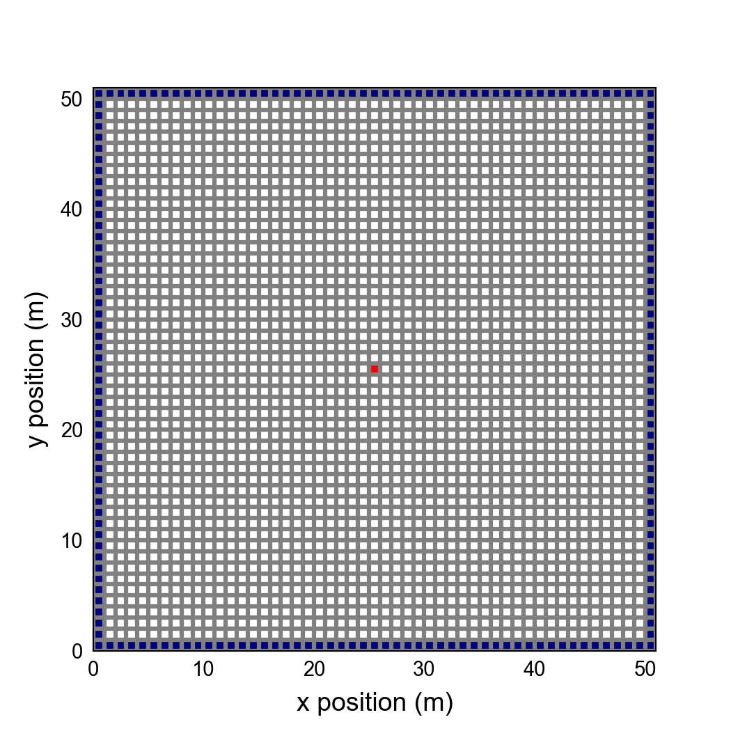
Figure 21.1 Model grid and boundary conditions used for the horizontal anisotropy problem. Blue cells are constant-head cells and the pumping well is located in the cell shown in red.
For this problem, hydraulic conductivity is anisotropic with K11 specified as 100 times larger than K22. For the first scenario the hydraulic conductivity ellipse is not rotated. For the second scenario, the ellipse is rotated 25 degrees counter clockwise in the horizontal plane. Because the ellipse axes do not align with the model grid, the XT3D option (Provost et al., 2017) is required to simulate this scenario. For the third scenario, the ellipse is rotated 90 degrees, so that groundwater flows more easily in the column direction.
Scenario |
Scenario Name |
Parameter |
Value |
|---|---|---|---|
1 |
ex-gwf-hanir |
angle1 |
0 |
xt3d |
False |
||
2 |
ex-gwf-hanix |
angle1 |
25 |
xt3d |
True |
||
3 |
ex-gwf-hanic |
angle1 |
90 |
xt3d |
False |
An initial head of zero was specified in all model cells. Constant head boundary cells with a value of zero were specified for all perimeter model cells. A pumping well with a rate of -1.0 \(m^3/d\) is located in the center of the model domain.
21.2. Scenario Results
Simulated drawdown for the three scenarios are shown in Figure 21.2, Figure 21.3, and Figure 21.4.
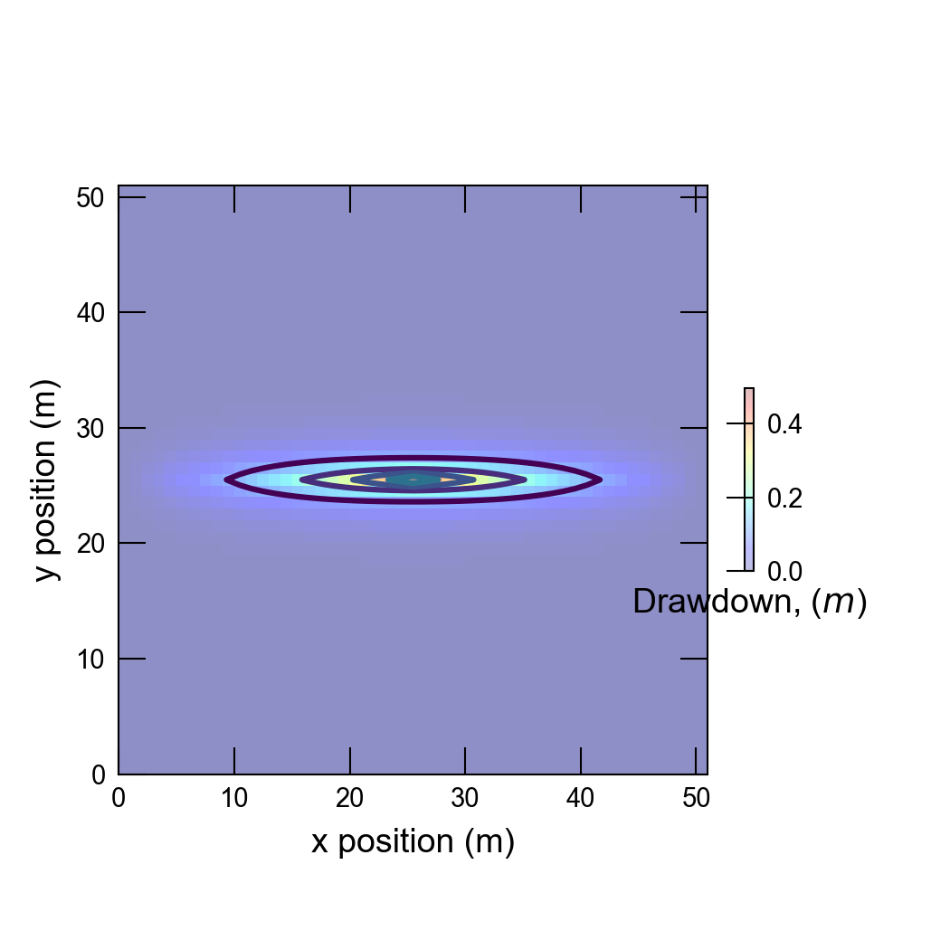
Figure 21.2 Simulated drawdown for anisotropic groundwater flow to a pumping well for scenario 1. The dominant hydraulic conductivity ellipse is aligned with the x-axis.
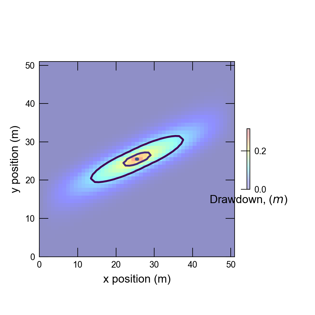
Figure 21.3 Simulated drawdown for anisotropic groundwater flow to a pumping well for scenario 2. The dominant hydraulic conductivity ellipse axis is rotated 25 degrees counter clockwise from the x-axis. The XT3D option is required for this scenario because the ellipse axes do not align with the row and column directions.
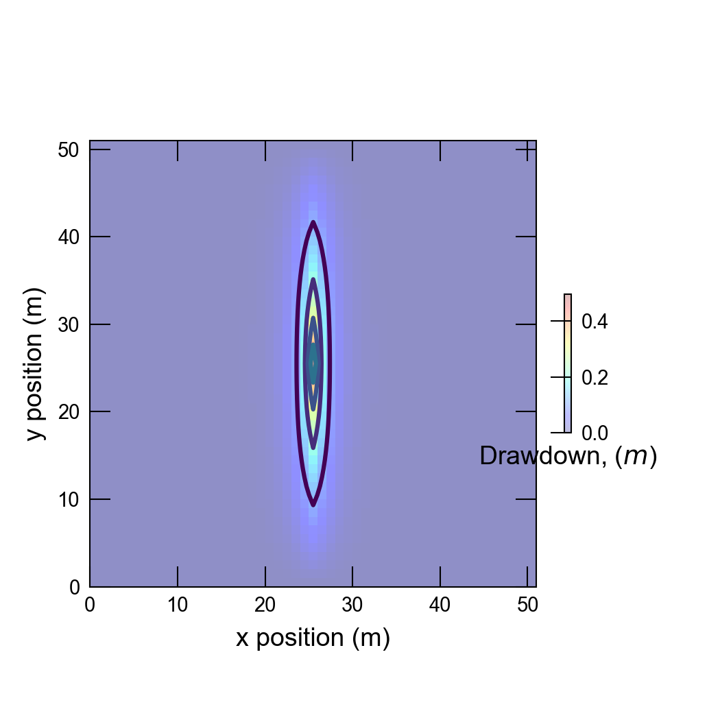
Figure 21.4 Simulated drawdown for anisotropic groundwater flow to a pumping well for scenario 3. The dominant hydraulic conductivity ellipse axis is rotated 90 degrees counter clockwise from the x-axis so that the ellipse axes align with the column and row directions.
21.3. References Cited
Provost, A. M., Langevin, C. D., & Hughes, J. D. (2017). Documentation for the “XT3D” Option in the Node Property Flow (NPF) Package of MODFLOW 6. https://doi.org/10.3133/tm6A56
21.4. Jupyter Notebook
The Jupyter notebook used to create the MODFLOW 6 input files for this example and post-process the results is: