61. Multipart Curvilinear Groundwater Flow Model
This example demonstrates how the MODFLOW 6 DISV Package can be used to simulate a multipart curvilinear model. This model extends the MODFLOW 6 “Curvilinear Groundwater Flow Model” example to reproduce the model grid presented in Figure 6 of (Romero & Silver, 2006). The hypothetical, curvilinear grid represents a meandering, curved flow path that traditional, structured grids cannot simulate. Figure 6 in (Romero & Silver, 2006) was introduced as an illustration of a curvilinear MODFLOW grid, but did develop it as a actual simulation model. This example illustrates that MODFLOW 6 can simulate this hypothetical grid.
61.1. Example Description
The hypothetical, curvilinear grid is composed of three distinct model regions that are combined to form the final grid. The first region (Left Grid; Figure 61.1A) is a curvilinear grid with 16 radial bands that start at 180\(^{\circ}\) and end at 270\(^{\circ}\) with a column discretization of 5\(^{\circ}\) (18 columns). The Left Grid’s inner- and outer-most radius is 4 \(ft\) and 20 \(ft\), respectively, and the radial direction vertices are 1 \(ft\) apart. The second region (Center Grid; Figure 61.1B) is a 1 \(ft\) rectangular, structured grid with 16 rows and 18 columns. The third region (Right Grid; Figure 61.1C) is an identical curvilinear grid as the first, but starts at 90\(^{\circ}\) and end at 0\(^{\circ}\). The three regions are combined to derive the hypothetical, curvilinear grid presented in Figure 61.2.
The hypothetical, curvilinear grid contains a single, 10 \(ft\) thick, model layer with a transmissivity of 0.19 \(ft^2/day\). There are two constant head boundary conditions that are placed along the columns of the curvilinear regions (Figure 61.2). The first constant head boundary is 10 \(ft\) and is along the first column of the Left Grid. The second constant head boundary is 3.334 \(ft\) and is along the last column of the Right Grid. The remaining model properties are summarized in Table 61.1.
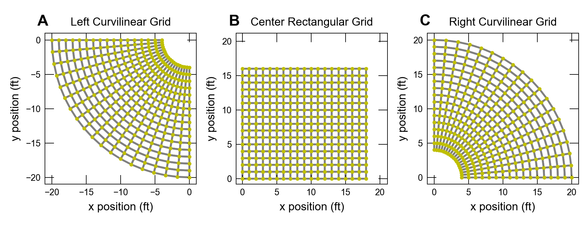
Figure 61.1 Three regions that combine to construct the hypothetical, curvilinear grid. A, Left curvilinear grid from 180\(^{\circ}\) to 270\(^{\circ}\), B, Center 16 by 18 rectangular grid , and C, Right curvilinear grid from 90\(^{\circ}\) to 0\(^{\circ}\). Grid vertices are marked in yellow. Note, the x, y coordinate positions are included for relative comparisons and not for the specific spatial location.
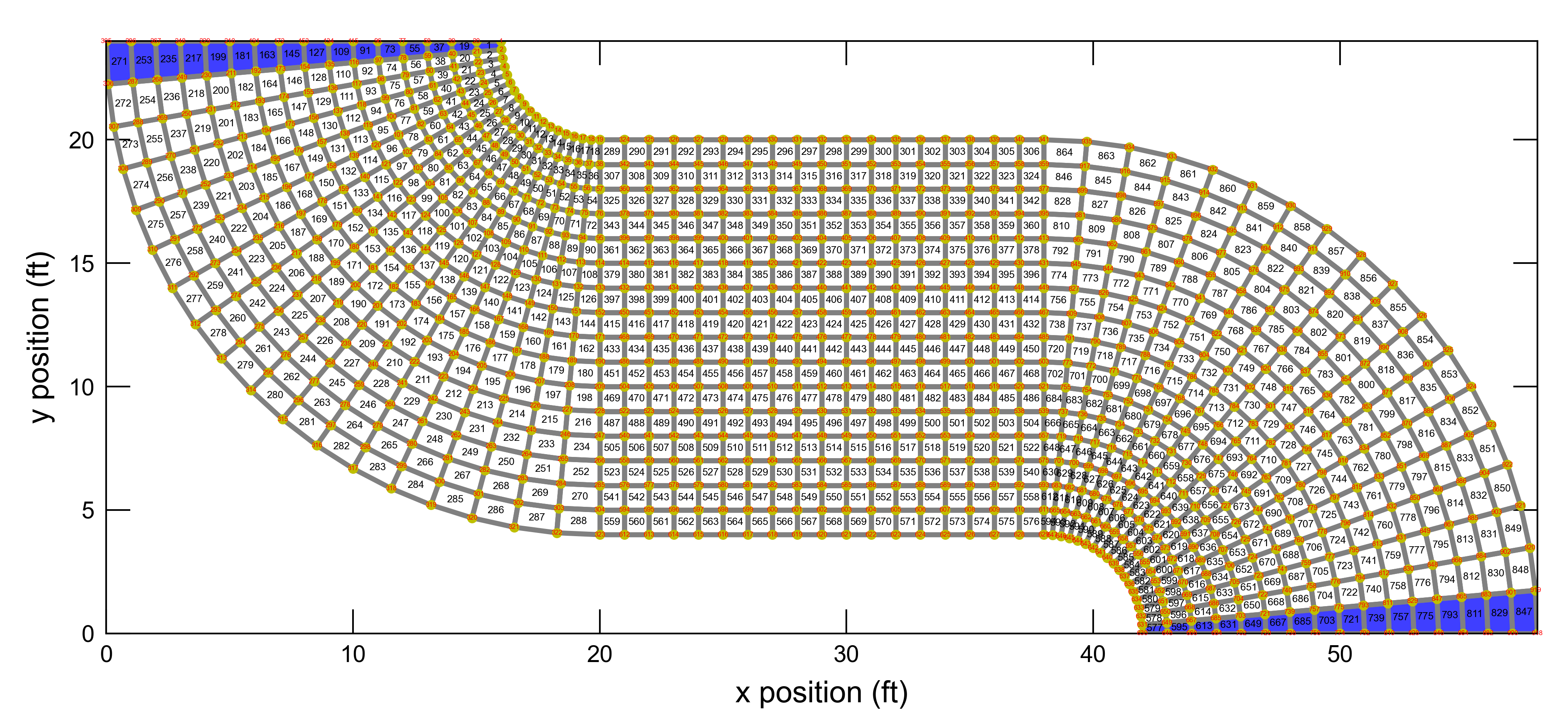
Figure 61.2 Plan view of the hypothetical, curvilinear grid with a meandering, curved flow path. Constant-head cells are marked in blue. The cell numbers \(1, 19, \ldots, 253, 271\) constant head is 10 \(ft\). The cell numbers \(577, 595, \ldots, 829, 847\) constant head is 3.33 \(ft\). Grid cell numbers are shown inside each model cell. Grid vertices are yellow with vertex numbers in red.
Parameter |
Value |
|---|---|
Simulation Type |
Steady–State |
Number of periods |
1 |
Number of time steps |
1 |
Number of layers |
1 |
Number cells per layer |
864 |
Top of the model (\(ft\)) |
10.0 |
Base of the model (\(ft\)) |
0.0 |
Horizontal transmissivity (\(ft^2/day\)) |
0.19 |
Horizontal hydraulic conductivity (\(ft/day\)) |
0.019 |
Left constant head boundary (\(ft\)) |
10 |
Right constant head boundary (\(ft\)) |
3.334 |
— Left Curvilinear Grid Properties — |
|
Degree angle of column 1 boundary |
180 |
Degree angle of column ncol boundary |
270 |
Degree angle width of each column |
5 |
Number of radial direction cells (radial bands) |
16 |
Number of columns in radial band (ncol) |
18 |
Grid inner radius (\(ft\)) |
4 |
Grid outer radius (\(ft\)) |
20 |
Radial band width (\(ft\)) |
1 |
— Middle Structured Grid Properties — |
|
Number of rows |
16 |
Number of columns |
18 |
Row width (\(ft\)) |
1 |
Column width (\(ft\)) |
1 |
— Right Curvilinear Grid Properties — |
|
Degree angle of column 1 boundary |
0 |
Degree angle of column ncol boundary |
90 |
Degree angle width of each column |
5 |
Number of radial direction cells (radial bands) |
16 |
Number of columns in radial band (ncol) |
18 |
Grid inner radius (\(ft\)) |
4 |
Grid outer radius (\(ft\)) |
20 |
Grid radial band width (\(ft\)) |
1 |
61.2. Example Results
- The hypothetical, curvilinear grid (fig.
Figure 61.2.) is solved using one, steady state,
stress period. Figure 61.3 presents the MODFLOW 6 simulated head and flow lines for all model cells.
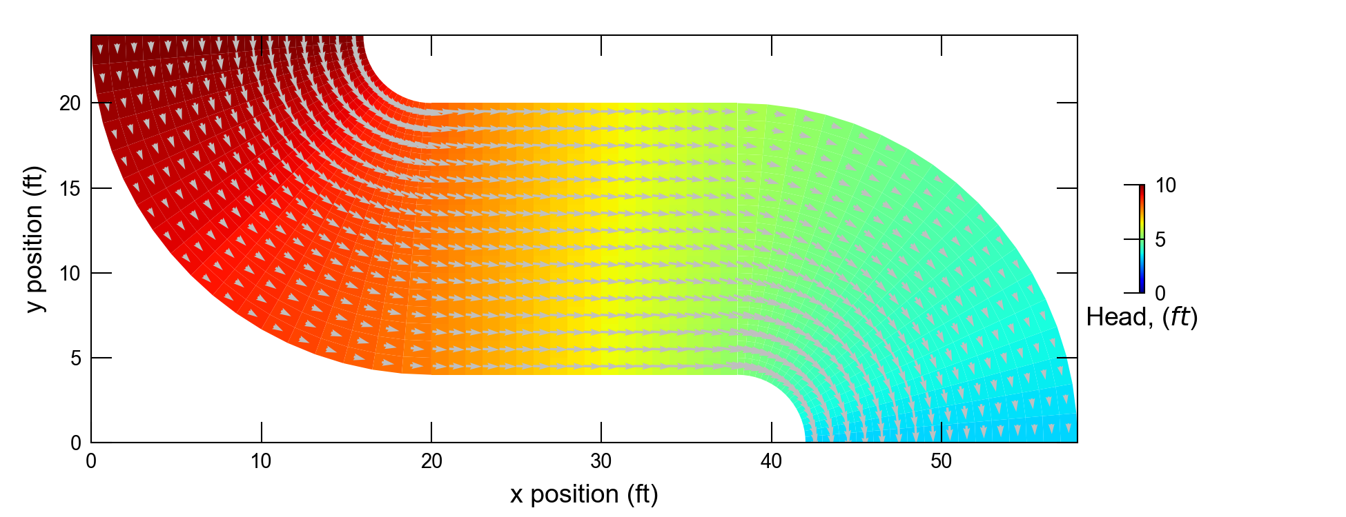
Figure 61.3 Steady state head solution and specific discharge vectors from the MODFLOW 6 curvilinear grid with a meandering, curved flow path.
61.3. References Cited
Romero, D. M., & Silver, S. E. (2006). Grid cell distortion and MODFLOW’s integrated finite-difference numerical solution. Groundwater, 44(6), 797–802. https://doi.org/10.1111/j.1745-6584.2005.00179.x
61.4. Jupyter Notebook
The Jupyter notebook used to create the MODFLOW 6 input files for this example and post-process the results is: