25. Laattoe Periodic Boundary Condition
This example shows how the exchange capability in MODFLOW 6 can be used to simulate spatial periodic boundary conditions (SPBC), such as the one described by (Laattoe et al., 2014). A SPBC can be used to represent spatially repeating groundwater flow conditions, such as those that might form beneath repeating bedforms on the sea floor. The example simulated here is equivalent to the first MODFLOW simulation reported by (Laattoe et al., 2014).
25.1. Example Description
The problem consists of a two-dimensional cross-section model consisting of 190 layers and 100 columns. Each cell is 0.06 \(m\) wide and each layer has a width of 0.03 \(m\). Model parameters are listed in Table 25.1.
Parameter |
Value |
|---|---|
Number of periods |
1 |
Number of layers |
190 |
Number of columns |
100 |
Number of rows |
1 |
Column width (\(m\)) |
0.06 |
Row width (\(m\)) |
1.0 |
Layer thickness (\(m\)) |
0.03 |
Top of the model (\(m\)) |
0.0 |
Starting head (\(m\)) |
0.0 |
Cell conversion type |
0 |
Horizontal hydraulic conductivity (\(m/d\)) |
1.0 |
An initial head of 0 \(m\) was specified for the model; however this model is not important as the model represents steady-state conditions.
The top of model has a constant-head condition assigned to layer 1. A different constant-head value is assigned to each cell based on a sine wave with an amplitude of 1.0 \(m\) and a wavelength of 6 \(m\), which is the length of the model in the x direction. The GWF-GWF Exchange is used to connect the cells on the left side of the model with the cells on the right side of the model. The first cell in each model cell is hydraulically connected to the last cell in each model layer. For example, the cell in (1, 1, 1) is hydraulically connected to the cell in (1, 1, 100). In MODFLOW 6, these cells are connected at the matrix solution level, rather than through outer iterations as was done by (Laattoe et al., 2014).
25.2. Example Results
Model results are shown in Figure 25.1. Groundwater flowing into cells on the left side of the model is instantaneously applied to cells on the right side of the model. Because the first column of cells is hydraulically connected to the last column of cell through the GWF-GWF Exchange, flow exiting the model through the left face automatically flows back into the model through the right face.
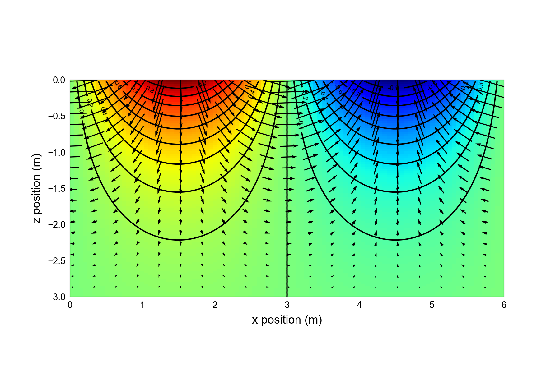
Figure 25.1 Cross section showing simulated head and vectors of specific discharge for the spatial periodic boundary condition example problem. Vectors of specific discharge are shown for every fifth cell in the layer and column directions.
25.3. References Cited
Laattoe, T., Post, V. E. A., & Werner, A. D. (2014). Spatial periodic boundary condition for MODFLOW. Groundwater, 52(4), 606–612. https://doi.org/10.1111/gwat.12086
25.4. Jupyter Notebook
The Jupyter notebook used to create the MODFLOW 6 input files for this example and post-process the results is: