25. CSUB Package Problem 2

This problem simulates the drainage of a thick interbed caused by a step decrease in hydraulic head in the aquifer and is based on sample problem 1 in (Hoffmann et al., 2003).

25.1. Theory

The equilibration of hydraulic heads in thick interbeds imbedded in an aquifer system typically lags head changes in the surrounding aquifer as a result of the characteristically low vertical hydraulic conductivity of fine-grained silts and clays that constitute the interbeds. Similarly, the hydraulic gradient within the interbeds can be treated as vertical if the horizontal extents of the interbeds are much greater than their thicknesses, the delayed dissipation of unequilibrated heads within the interbeds can be described by the one-dimensional diffusion equation,

(25.1)\[\frac{\partial ^2 h}{\partial z^2} = \frac{S^{\prime}_{S}}{K^{\prime}_{v}} \frac{\partial h}{\partial t},\]

where \(z\) is the vertical spatial coordinate (L), \(S^{\prime}_{S}\) is the specific storage of the interbed (unitless), \(K^{\prime}_{v}\) is the vertical hydraulic conductivity of the interbed (L/T), and \(t\) is time (T). The solution of this diffusion problem is identical to heat diffusion. (Carslaw & Jaeger, 1959) developed an analytical solution for heat diffusion from a slab with the ends at a constant temperature that can be recast to solve equation 25.1 for delayed flow from a thick interbed. If the initial head at \(t = 0\) is \(h_0\) throughout the thickness of the interbed (\(b_0\)), and the head in the surrounding aquifer is \(\Delta h\) above \(h_0\) for \(t > 0\), the head distribution \([h(z, t)]\) for the interbed can be written as the infinite series

(25.2)\[h(z, t) - h_0 = \Delta h - \frac{4 \Delta h}{\pi} \sum^{\infty}_{k = 0} \frac{-1^k}{2k + 1} e^{-\frac{\pi^2}{4} \frac{t}{\tau_k}} \cos \left( \frac{(2k + 1) \pi z}{b_0} \right),\]

where the time constant, \(\tau_k\), is defined as

(25.3)\[\tau_k = \frac{ \left( \frac{b_0}{2} \right)^2 S^{\prime}_{S} }{\left( 2k + 1 \right)^2 K^{\prime}_{v}}.\]

In equation 25.2, \(z = 0\) is assumed to be at the midplane of the interbed, with the boundaries at \(\pm \frac{b_0}{2}\). Note that both the coefficients in the sum and the \(\tau_k\) decrease as \(k\) increases. Thus, the true head distribution can be adequately described by a finite number of addends (\(k\)), particularly for later times. In the context of interbed compaction and land subsidence, the time delay caused by slow dissipation of transient overpressures is often given in terms of the time constant

(25.4)\[\tau_0 = \frac{ \left( \frac{b_0}{2} \right)^2 S^{\prime}_{S} }{K^{\prime}_{v}},\]

which is the time during which about 93 percent of the ultimate compaction for a given decrease in head occurs (Riley, 1969). Because \(\tau_0\) is proportional to \(S^{\prime}_{S}\), which generally is much larger for inelastically deforming interbeds than for elastically deforming interbeds, deformation in elastically deforming interbeds is often assumed to occur instantaneously. The same is true for very thin inelastically deforming interbeds. Thus, equation 25.4 can be used to determine in which interbeds the time constant exceeds the model time step, necessitating consideration of use of delay-interbeds, which account for delayed drainage processes, instead of no-delay interbeds.

Under constant geostatic stress conditions, compaction in the interbed can be directly related head changes using

(25.5)\[\Delta b = S^{\prime}_{S} \Delta h,\]

where \(\Delta b\) is the change in thickness of the interbed (L).

25.2. Example Description

Static model parameters are summarized in Table 25.1. The model grid for this problem consists of 1 layer, 1 row, and 3 columns (Figure 25.1). The model has a top elevation of 0 meters and bottom elevation of -1,000 meters. DELR and DELC are equal to 1 meter. The simulation consists of one transient stress period 1,000 days in length, and is divided into 100 variable length time steps calculated using a time step multiplier equal to 1.05.

Table 25.1 Model parameters for example ex-gwf-csub-p02.

Parameter	Value
Number of periods	1
Number of layers	1
Number of columns	3
Number of rows	1
Column width (\(m\))	1.0
Row width (\(m\))	1.0
Top of the model (\(ft\))	0.0
Layer bottom elevations (\(m\))	–1000.0
Starting head (\(m\))	0.0
Cell conversion type	0
Horizontal hydraulic conductivity (\(m/d\))	1.0e6
Specific gravity of moist soils (unitless)	1.7
Specific gravity of saturated soils (unitless)	2.0
Interbed drainage time constant (unitless)	1000.0
Coarse-grained material porosity (unitless)	0.2
Elastic specific storage (\(1/m\))	1.0e-5
Inelastic specific storage (\(1/m\))	1.0e-2
Interbed porosity (unitless)	0.45
Initial interbed head (\(m\))	1.0
Initial preconsolidation head (\(m\))	1.0

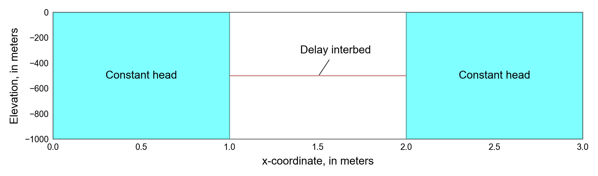
Figure 25.1 Model domain and setup for the delay interbed drainage problem. Interbed drainage is the result of step decrease in head in the aquifer

The hydraulic conductivity in the aquifer was set to a very large value (1 × 10⁶ meters per day), so that the head in the aquifer in the center cell remains constant. The specific yield and specific storage in the STO package were set to 0. Default flow property (NPF) and storage (STO) package settings were used. Initial heads were specified to be 0 meters.

25.2.1. Head-Based Formulation

Initially, the head-based formulation of the CSUB package was used to simulate compaction of the delay interbed and compare to analytical results calculated using equations 25.2 and 25.5 (Table 25.2). Ten finite-difference nodes represent the half-thickness of the interbed. The time constant, \(\tau_0\) (eq. 25.4), was chosen to be 1,000 with vertical hydraulic conductivity set to 2.5 × 10⁻⁶ meters per day, interbed thickness set to 1 meters, and elastic skeletal specific storage set to 1 × 10⁻⁵ per meter and inelastic skeletal specific storage set to 0.01 per meter. Meters and days units have been used in this problem but any consistent set of length and time units results in the same solution. The specific storage of coarse-grained aquifer material were specified to be 0 × 10⁻⁶ per meter. Water compressibility was not simulated in this problem and the thickness of compressible materials and total porosity were not updated during the simulation.

Table 25.2 Scenario parameters for example ex-gwf-csub-p02.

Scenario	Scenario Name	Parameter	Value
1	e x-gwf-csub-p02a	head based	True
		bed thickness	(1.0,)
		kv	(2.5e-06,)
		ndelaycells	19
2	e x-gwf-csub-p02b	head based	False
		bed thickness	(1.0,)
		kv	(2.5e-06,)
		ndelaycells	19
3	e x-gwf-csub-p02c	head based	True
		bed thickness	(1.0, 2.0, 5.0, 10.0, 20.0, 50.0, 100.0)
		kv	(2.5e-06, 1e-05, 6.25e-05, 0.00025, 0.001, 0.00625, 0.025)
		ndelaycells	1001

Constant-head cells, with a value of 0 meters, bound the delay interbed in column 2. The water released from the interbed during the simulation can leave the system through these constant-head cells. The starting head and the preconsolidation head in the delay interbed were specified to be 1 meter higher than the initial head in the surrounding aquifer.

The resulting compaction of the interbed is compared to the analytical solution (derived using equations 25.2, 25.4, and 25.5) in Figure 25.1. The CSUB-computed values closely match the analytical values. The small differences, particularly at early times, may be at least partly due to the fact that the aquifer head in the simulation does not remain exactly constant as a result of water entering the aquifer from the interbed. Because of the finite transmissivity of the aquifer, the head in the aquifer briefly rises to about 2 percent of the starting head in the interbed during the first time step.

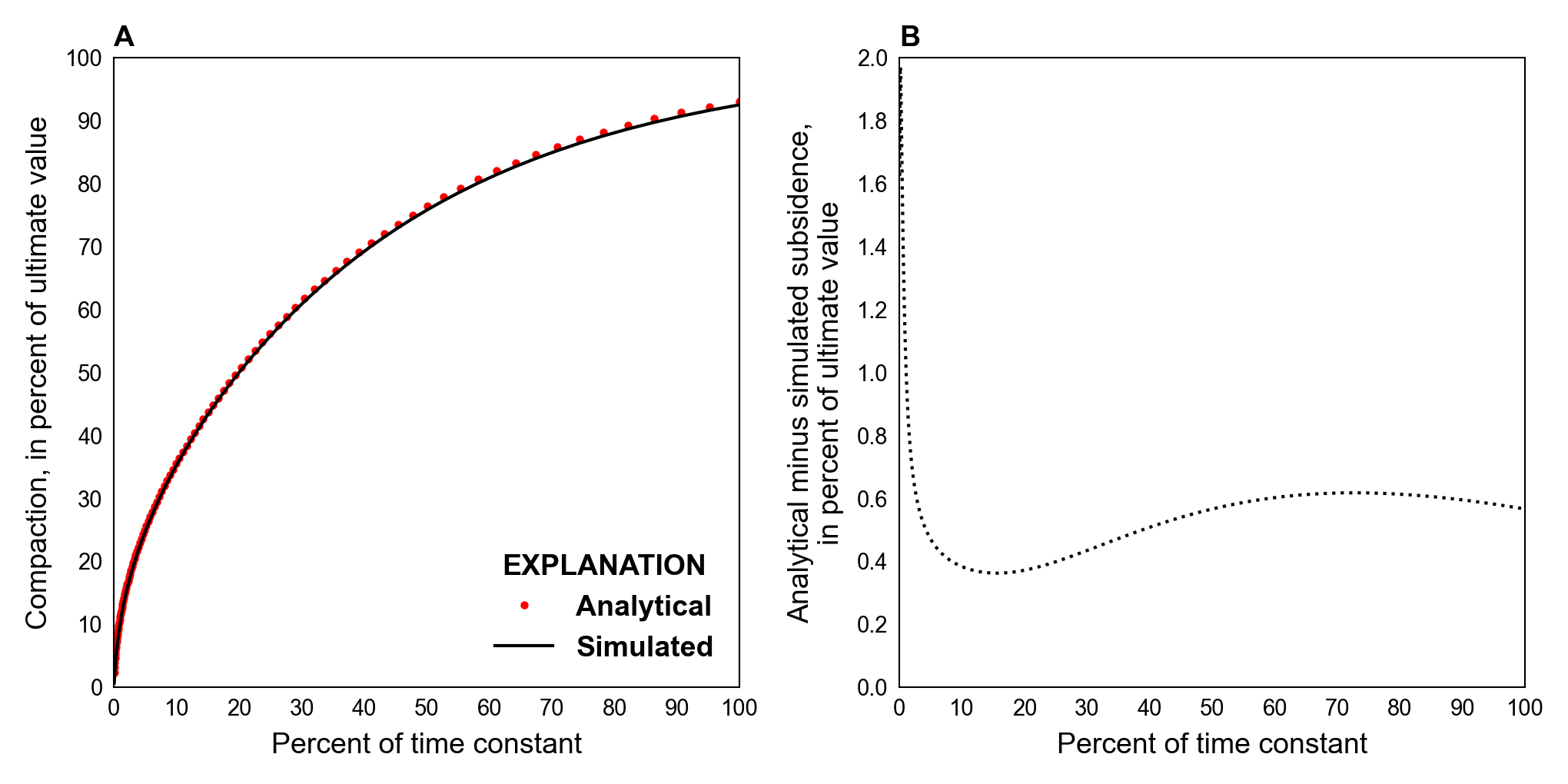
Figure 25.2 Graphs showing comparisons of simulated compaction with the head-based formulation and the analytical solution for the delay interbed drainage problem. A, comparison of the compaction history simulated with the analytical solution to the problem, and B, difference between the analytical solution and simulated compaction

25.2.2. Effective Stress-Based Formulation

To evaluate differences between the head- and effective stress-based formulations, the problem shown in Figure 25.1 was modified to use the effective stress-formulation (Table 25.2). A total of 19 finite-difference nodes were used in the effective stress-based formulation so that results could be directly compared to the head-based formulation that used 10 finite-difference cells to represent the half-thickness of the interbed. A specific gravity of 1.7 and 2.0 was defined for moist and saturated sediments, respectively. The initial preconsolidation stress was set to be 1 meter less than the initial effective stress of 1,000 meters and is based on the initial preconsolidation head, which was defined to be 1 meter above the initial head in the head-based formulation.

The resulting effective stress-based compaction of the interbed is compared to the head-based solution in Figure 25.3. The effective stress-based values closely match the head-based values. The small differences (\(<\) 0.1%) are partly due to the fact that calculated specific storage values are not constant in the effective stress-formulation. Furthermore, the inelastic and elastic compression indices (41.8 and 4.18 × 10⁻² (unitless)), respectively), which are internally calculated from the initial effective stress and the user-provided inelastic and elastic specific storage values, results in a slightly smaller initial inelastic storativity value (9.5 × 10⁻³ versus 1.0 × 10⁻²) that increase to values slightly larger than the user-provided inelastic storativity in subsequent time steps.

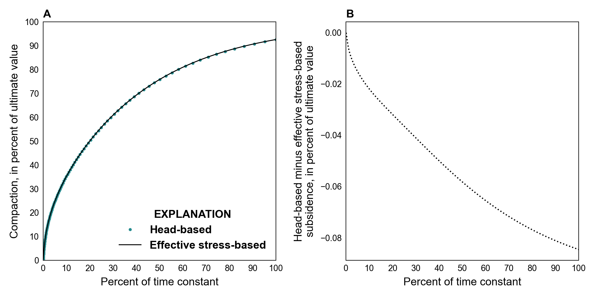
Figure 25.3 Graphs showing comparisons of simulated compaction for head- and effective stress-based formulations for the delay interbed drainage problem. A, comparison of the compaction history simulated with the head- and effective stress-based formulation solution to the problem, and B, difference between the simulated head- and effective stress-based formulation compaction

Another reason the difference between the head- and effective stress-based compaction shown in Figure 25.3 is small is the interbed thickness is small (1 meter) and as a result the difference between the effective stress at the top and bottom of the interbed is also small.

25.2.3. Effect of Interbed Thickness on the Effective Stress-Based Formulation

To evaluate the effect of the interbed thickness affects compaction, head- and effective stress-based models were run with interbed thicknesses ranging from 1 to 100 m (Table 25.2). A time constant (\(\tau_0\)) of 1,000 was used with elastic and inelastic skeletal specific storage values of 1 × 10⁻⁵ and 0.01 per meter, respectively, were used for each interbed thickness evaluated. The vertical hydraulic conductivity for each interbed thickness evaluated was calculated using equation 25.3 and the specified \(\tau_0\) and specific storage values. The calculated vertical hydraulic conductivity ranged from 2.5 × 10⁻⁶ to 0.025 meters per day for interbed thickness ranging from 1 to 100 meters, respectively. A total of 1,001 finite-difference nodes were used to simulate the interbed for the head- and effective stress-based formulation simulations to provide additional spatial resolution for simulated interbed heads; the head-based simulations were simulated using a full-cell formulation. All other model parameters for the simulations that evaluated different interbed thicknesses were unchanged from the original values.

The difference between the analytical and simulated compaction and drainage rates at the top and bottom of the interbed relative to analytical drainage rates are shown in Figure 25.4. The difference between head- and effective stress-based compaction for a 1 meter interbed thickness shown in Figure 25.4A are identical to the results shown in Figure 25.3B. In general, the differences between the simulated results and the analytical solution are comparable for interbed thickness less than 20 meters. Coincident with compaction differences, the average difference in drainage from the top and bottom of the interbed to the aquifer is greater than 0.7% (Figure 25.4B) for interbed thicknesses greater than 10 meters as a result of larger differences in the effective stress at the top and bottom of the interbed. The average difference between the effective stress at the bottom and top of the interbed is 2.02%, 5.13%, and 10.5% of the average interbed effective stress for the simulations with 20, 50, and 100 meters interbed thicknesses, respectively.

Figure 25.5 shows the vertical distribution of the difference in head- and effective stress-based formulation interbed heads relative to head-based interbed heads for each of the interbed thicknesses evaluated. Head-based interbeds heads are symmetric about the center line of the interbed, with lower heads at the top and bottom of the interbed and the highest heads at the center of the interbed. As a result, negative and positive differences shown in Figure 25.5 represent higher and lower interbed heads in the effective stress-based formulation than the head-based formulation, respectively. Generally, effective stress-based interbed heads are higher and lower in the top and bottom halves of the interbed, respectively, and differences are greatest for interbed thicknesses greater than 10 meters. The spatial distribution of interbed head differences is controlled by the decrease in the inelastic specific storage value resulting from the increase in effective stress with depth and the reduction in the water released from storage with depth in the interbed, which results in increased head changes with depth with the effective stress-formulation. As the simulation progresses, differences propagate from the top and bottom of interbed into the interbed as the maximum difference decreases.

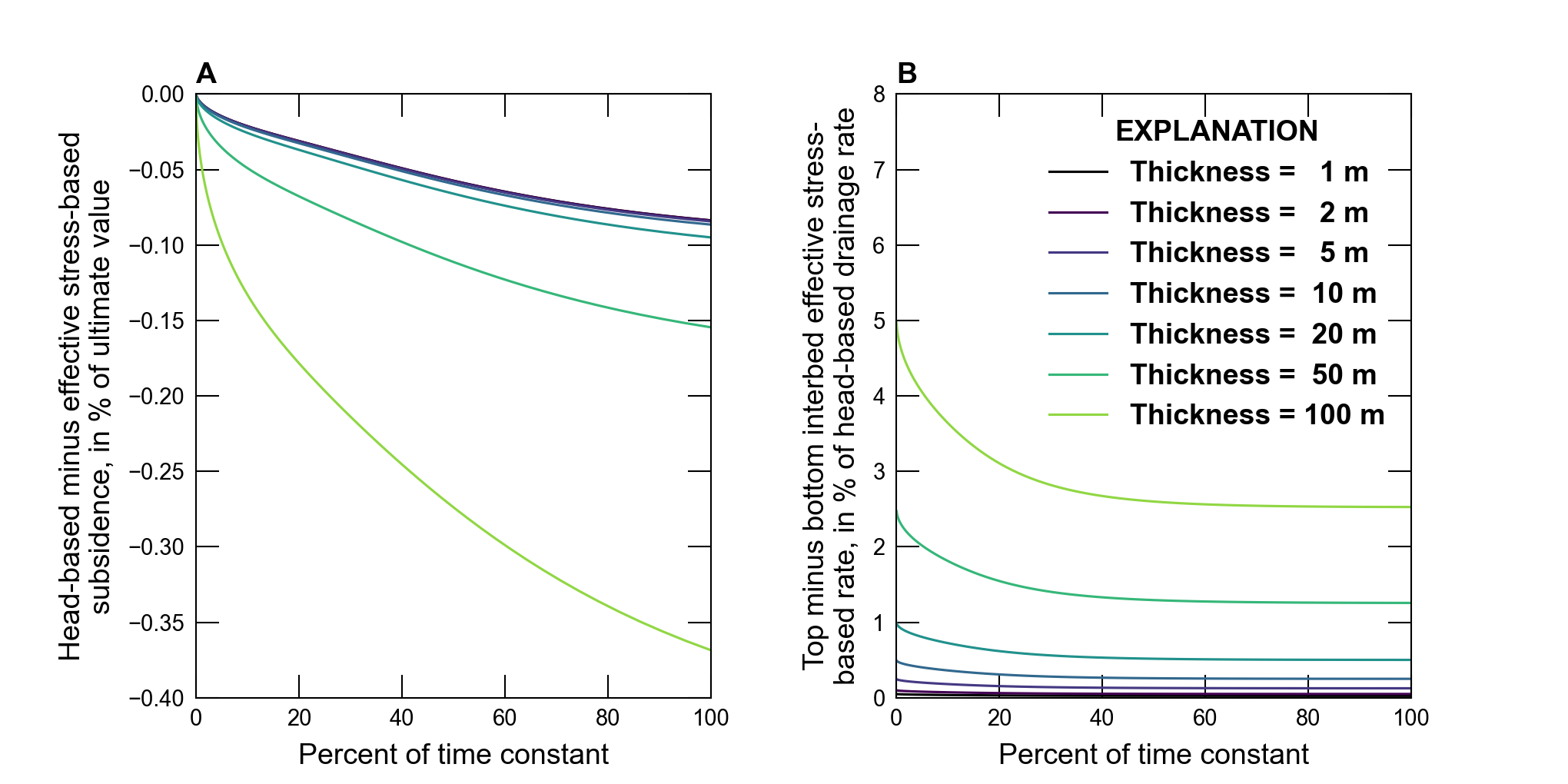
Figure 25.4 Graphs showing the difference between head- and effective stress-based compaction for different interbed thicknesses for the delay interbed drainage problem. A, difference between the head- and effective stress-based formulation compaction, and B, difference between drainage at the top and bottom of the interbed relative to the head-based formulation interbed drainage

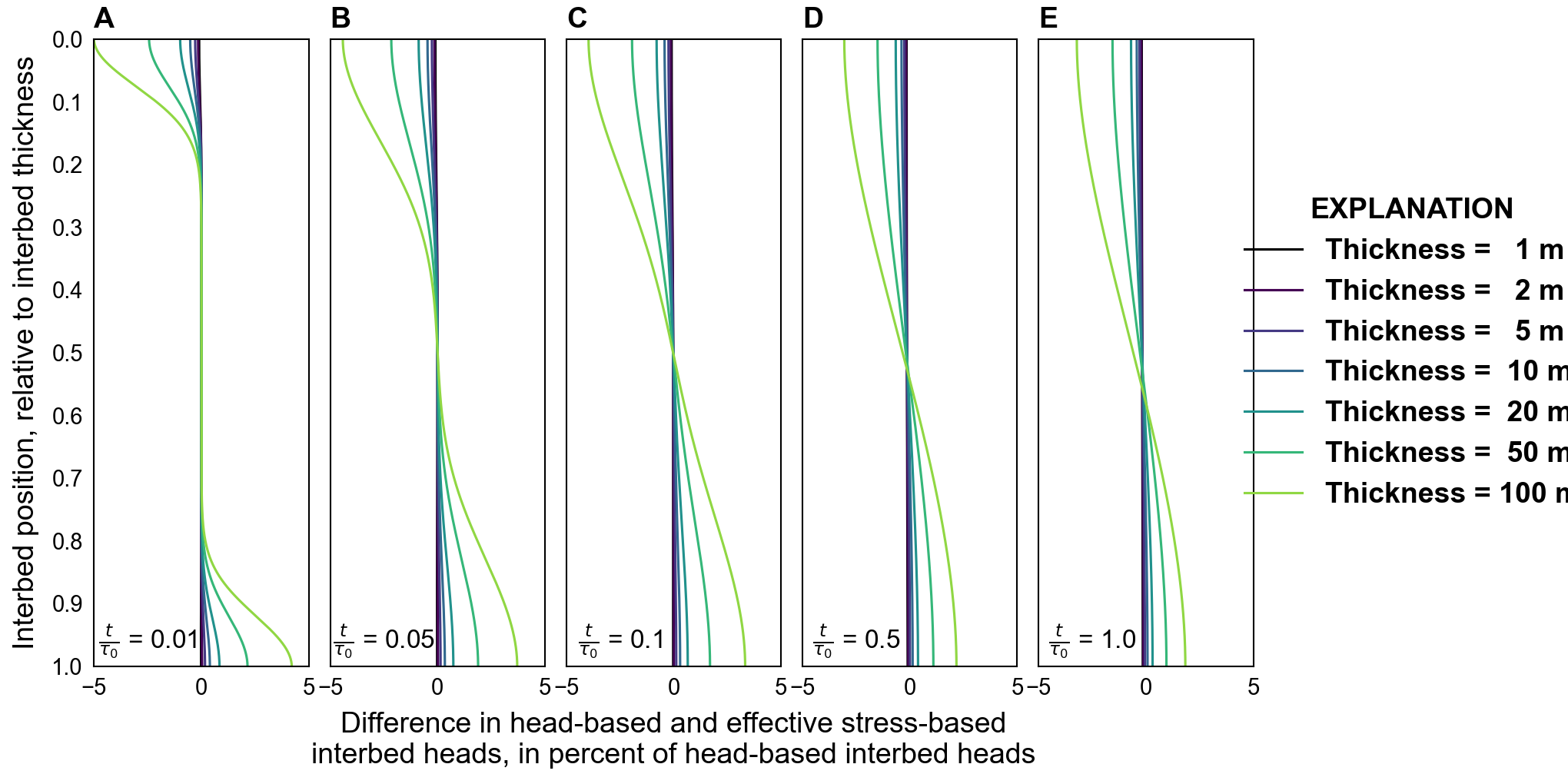
Figure 25.5 Graphs showing differences between head- and effective stress-based formulation interbed heads relative to head-based interbed heads for variable interbed thicknesses at select fractions of the time constant (\(\tau_0\)) for the delay interbed drainage problem. A, 1 percent of \(\tau_0\), B, 5 percent of \(\tau_0\), C, 10 percent of \(\tau_0\), D, 50 percent of \(\tau_0\), and E, 100 percent of \(\tau_0\)

25.3. References Cited

Carslaw, H. S., & Jaeger, J. C. (1959). Conduction of heat in solids. Oxford: Clarendon Press, 1959, 2nd Ed.

Hoffmann, J., Leake, S. A., Galloway, D. L., & Wilson, A. M. (2003). MODFLOW-2000 Ground-Water Model—User Guide to the Subsidence and Aquifer-System Compaction (SUB) Package. Retrieved from https://pubs.usgs.gov/of/2003/ofr03-233/

Riley, F. S. (1969). Analysis of borehole extensometer data from Central California. International Association of Scientific Hydrology Publication 89, 2, 423–431.

25.4. Jupyter Notebook

The Jupyter notebook used to create the MODFLOW 6 input files for this example and post-process the results is:

• ex-gwf-csub-p02