41. MT3DMS Problem 5
The next example problem tests two-dimensional transport in a radial flow field. The radial flow field is established by injecting water in the center of the model domain (row 16, column 16) and allowing it to flow outward toward the model perimeter. No regional groundwater flow gradient exists as in some of the previous comparisons with MT3DMS. Constant head cells located around the perimeter of the model drain water and solute from the simulation domain. Solute enters the model domain through the injection well with a unit concentration. The starting concentration is zero across the entire domain. Flow remains steady and confined throughout the 27 day simulation period. The aquifer is homogeneous, isotropic, and boundaries are sufficiently far from the injection well to avoid solute reaching the boundary during the simulation interval. Table 41.1 summarizes many of the model inputs:
Parameter |
Value |
|---|---|
Number of layers |
1 |
Number of rows |
31 |
Number of columns |
31 |
Column width (\(m\)) |
10.0 |
Row width (\(m\)) |
10.0 |
Layer thickness (\(m\)) |
1.0 |
Top of the model (\(m\)) |
0.0 |
Porosity |
0.3 |
Simulation time (\(days\)) |
27 |
Horizontal hydraulic conductivity (\(m/d\)) |
1.0 |
Volumetric injection rate (\(m^3/d\)) |
100.0 |
Concentration of injected water (\(mg/L\)) |
1.0 |
Longitudinal dispersivity (\(m\)) |
10.0 |
Ratio of transverse to longitudinal dispersitivity |
1.0 |
Molecular diffusion coefficient (\(m^2/d\)) |
1.0e-9 |
An analytical solution for this problem was originally given in (Moench & Ogata, 1981). The MT3DMS solution with the TVD option activated most closely matched the analytical solution. Therefore the TVD option is activated in both MT3DMS and MODFLOW 6 for verifying the transport solution. Figure 41.1 shows a slight under simulation of the outward spread of solute in the MODFLOW 6 solution compared to MT3DMS. Figure Figure 41.2 shows close agreement among the MT3DMS and MODFLOW 6 isoconcentration contours with the TVD advection scheme activated.
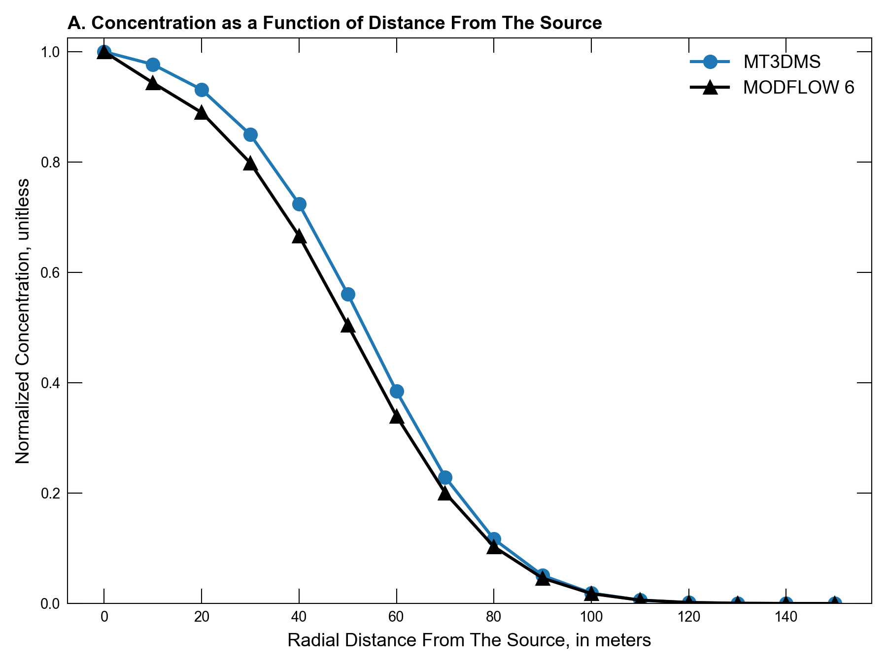
Figure 41.1 Comparison of the MT3DMS and MODFLOW 6 numerical solutions for a point source in a two-dimensional radial flow field simulation. The thick black line in Figure 41.2 shows the location of this profile view of concentrations. The analytical solution for this problem was originally given in (Moench & Ogata, 1981) and is not shown here
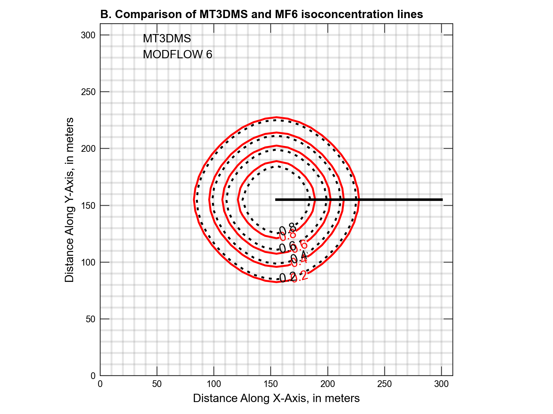
Figure 41.2 Comparison of the MT3DMS and MODFLOW 6 numerical solutions for two-dimensional transport in a radial flow field. The thick black line shows the location of the concentration profile shown in Figure 41.1. Both models are using their respective finite difference solutions with the use of the TVD option.
41.1. References Cited
Moench, A., & Ogata, A. (1981). A numerical inversion of the Laplace transform solution to radial dispersion in a porous medium. Water Resources Research, 17(1), 250–252. https://doi.org/10.1029/WR017i001p00250
41.2. Jupyter Notebook
The Jupyter notebook used to create the MODFLOW 6 input files for this example and post-process the results is: