33. Keating Problem
This example is based on an unsaturated flow and transport problem described in (Keating & Zyvoloski, 2009) under the section “Extension to Mixed Vadose/ Saturated Zone Simulations.” The problem consists of a two-dimensional cross-section model with a perched aquifer overlying a water table aquifer. This problem offers a difficult test for the Newton flow formulation in MODFLOW 6 as well as for the transport model, which must transmit solute through dry cells. This problem was also used by (Bedekar et al., 2016) as a test for their solute routing approach implemented in MT3D-USGS for flow models solved with MODFLOW-NWT (Niswonger et al., 2011).
In addition to the transport model, this example also includes a particle tracking model. The model demonstrates the default approach taken by MODFLOW 6 to track particles through dry cells under the Newton formulation, which is to drop the particles instantaneously to the top-most active cell in the vertical column and resume tracking as usual.
33.1. Example description
The parameters used for this problem are listed in Table 33.1. The model grid consists of 1 row, 400 columns, and 80 layers. The flow problem consists of a perched aquifer overlying an unconfined water table aquifer. A perched aquifer forms due the presence of a thin, discontinuous low permeability lens located near the center of the model domain. Flow conditions are simulated as steady state. The solute transport simulation represents transient conditions, which begin with an initial concentration specified as zero everywhere within the model domain. For the first 730 days, recharge enters at a concentration of one. For the remainder of the simulation, recharge has a solute concentration of zero.
Constant-head conditions are prescribed on the left and right sides of the model with head values of 800 \(m\) and 100 \(m\), respectively. These constant-head conditions are only assigned if the cell bottom elevation is below the prescribed head value. Water entering the model from the constant head cells is assigned a concentration of zero. Water leaving the constant head cells on the right side of the model leaves at the simulated concentration in the cell.
The Newton formulation is used to simulate flow through the domain. Recharge is assigned to the top of the model, and although upper model cells are dry, this recharge water is instantaneously transmitted down to the perched aquifer. The perched aquifer flows to the left and right and spills over the edges of the confining unit. Water flowing over the edges instantaneously recharges the underlying water table aquifer. A negligible amount of water flows through the low permeability lens and then down into the water table aquifer. The flow problem is challenging to solve and converges best with backtracking, under relaxation, and solver parameters designed for complex problems.
For the transport model, the simulation period is divided into 3000, 10-day time steps. Advection and dispersion are simulated. Because the longitudinal and transverse dispersivities are equal, the computationally demanding XT3D approach is not needed to represent dispersion. The simpler method for calculating dispersion is used instead, and gives comparable results to those obtained with XT3D.
Parameter |
Value |
|---|---|
Number of layers |
80 |
Number of rows |
1 |
Number of columns |
400 |
Column width (\(m\)) |
25.0 |
Row width (\(m\)) |
1.0 |
Layer thickness (\(m\)) |
25.0 |
Top of model domain (\(m\)) |
2000.0 |
Bottom of model domain (\(m\)) |
0.0 |
Permeability of aquifer (\(m^2\)) |
1.0e-12 |
Permeability of aquitard (\(m^2\)) |
1.0e-18 |
Head on left side (\(m\)) |
800.0 |
Head on right side (\(m\)) |
100.0 |
Recharge (\(kg/s\)) |
0.5 |
Normalized recharge concentration (unitless) |
1.0 |
Longitudinal dispersivity (\(m\)) |
1.0 |
Transverse horizontal dispersivity (\(m\)) |
1.0 |
Transverse vertical dispersivity (\(m\)) |
1.0 |
Length of first simulation period (\(d\)) |
730 |
Length of second simulation period (\(d\)) |
29270.0 |
Porosity of mobile domain (unitless) |
0.1 |
Layer, row, and column for observation 1 |
(49, 1, 119) |
Layer, row, and column for observation 2 |
(77, 1, 359) |
33.2. Example Results
Simulated heads from MODFLOW 6 are shown in Figure 33.1. Cells with a calculated head beneath the cell bottom are considered “dry” and are not shown with a color. The zone of recharge is shown in red on the top of the plot.
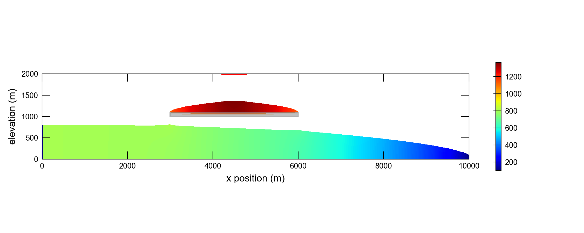
Figure 33.1 Color shaded plot of heads simulated by MODFLOW 6 for the (Keating & Zyvoloski, 2009) problem involving groundwater flow and transport through an unsaturated zone. Recharge is applied to the narrow strip shown in red on the top of the model domain.
Simulated concentrations from MODFLOW 6 are shown in Figure 33.2 for three different times. These plots show the development of the solute plume in the perched aquifer, and then shows flushing of the perched aquifer when the recharge concentration becomes zero. In the underlying water table aquifer, two solute plumes are formed as groundwater flows over the edges of the low permeability lens. These plumes then flow toward the right, and eventually exit through the constant head cells. Plots of concentration versus time for the two yellow points shown in Figure 33.2 are shown in Figure 33.4. Results from MODFLOW 6 are shown with the results presented by (Keating & Zyvoloski, 2009) and are in good agreement considering the complexity of the problem. Similar plots for this problem are also presented by (Bedekar et al., 2016).
Simulated particle tracks from MODFLOW 6 are shown in Figure 33.3. A particle is released at the center of every cell in the top layer of the grid. Particle pathlines are colored such that adjacent pathlines may be easily distinguished.
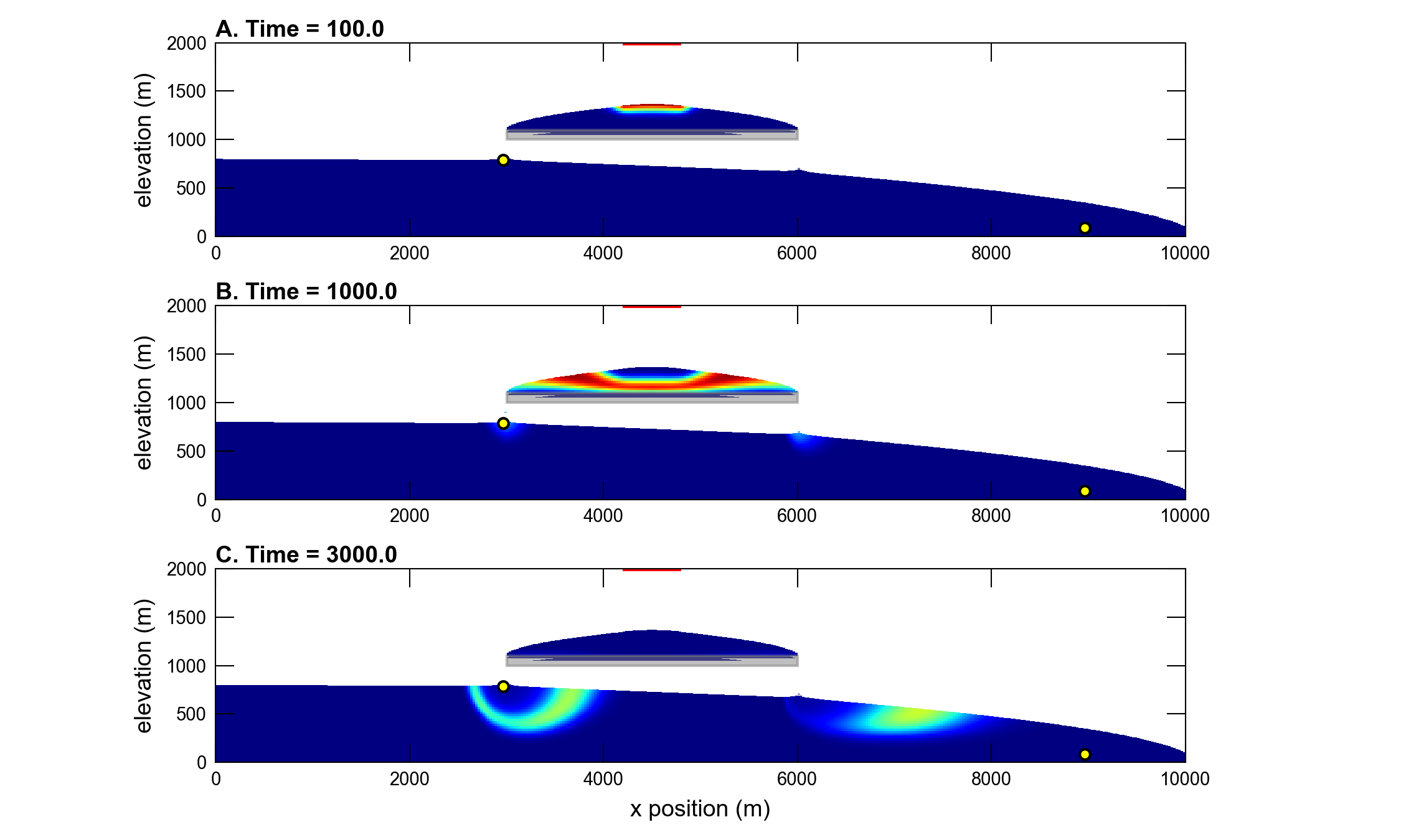
Figure 33.2 Color shaded plots of concentrations simulated by MODFLOW 6 for the (Keating & Zyvoloski, 2009) problem involving groundwater flow and transport through an unsaturated zone. This plot can be compared to figure 11 in (Bedekar et al., 2016), which shows similar plots for MT3D-USGS results. Plots of concentration versus time are shown in Figure 33.4 for the two points shown in yellow.

Figure 33.3 Particle pathlines simulated by MODFLOW 6 for the (Keating & Zyvoloski, 2009) problem involving groundwater flow and transport through an unsaturated zone. A particle is released at the center of each recharge cell in the top layer of the grid.
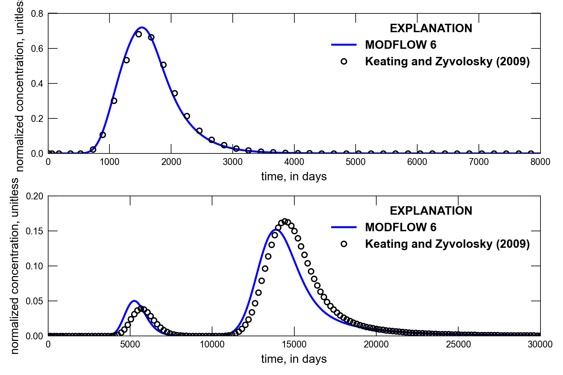
Figure 33.4 Concentrations versus time for two observation points as simulated by MODFLOW 6 and by (Keating & Zyvoloski, 2009) for a problem involving groundwater flow and transport through an unsaturated zone. This plot can be compared to figure 12 in (Bedekar et al., 2016), which shows a similar plot for MT3D-USGS results.
33.3. References Cited
Bedekar, V., Morway, E. D., Langevin, C. D., & Tonkin, M. J. (2016). MT3D-USGS version 1: A U.S. Geological Survey release of MT3DMS updated with new and expanded transport capabilities for use with MODFLOW. https://doi.org/10.3133/tm6a53
Keating, E., & Zyvoloski, G. (2009). A stable and efficient numerical algorithm for unconfined aquifer analysis. Ground Water, 47(4), 569–579. https://doi.org/10.1111/j.1745-6584.2009.00555.x
Niswonger, R. G., Panday, S., & Ibaraki, M. (2011). MODFLOW-NWT, A Newton formulation for MODFLOW-2005. Retrieved from https://pubs.er.usgs.gov/publication/tm6A37
33.4. Animation
Animation of model results: