73. Thermal Profile along a Particle Path
This example demonstrates the simultaneous use of three different model types in MODFLOW 6: (1) groundwater flow (GWF), (2) groundwater energy transport (GWE), and (3) particle transport (PRT). Both GWF and GWE solve for steady flow and temperature conditions, respectively. PRT is used to route two particles through the steady flow and heat transport fields and once informed of the particle locations through time, each x-y location is mapped to a temperature that is then plotted.
73.1. Example description
A Voronoi model grid is simulated with the discretization by vertices package (DISV). The simulation domain is 2,000 \(m\) by 1,000 \(m\) and is used by all three model types mentioned above. In the flow model, arbitrarily configured specified head boundaries around the perimeter of the model are as follows: the left-hand boundary is set to 2.0 m, the bottom boundary cells are set to 1.8 m, and the right-hand boundary is set to 1.0 m. Two extraction wells are located in the model domain with the host cells shaded red (Figure 73.1). One is located near the lowerleft of the domain and the second extraction well is located just right of the center of the simulation domain. One injection well is located near the upper right portion of the active domain with the host cell also shaded red (Figure 73.1).
The GWE model uses a standard set of thermal parameters listed in Table 73.1. A thermal gradient along the left-hand boundary and is setup such water entering the domain in the lower left corner starts at 0.0 \(^{\circ}C\) with a linear gradient increasing to 100.0 \(^{\circ}C\) in the uppper-left corner of the simulation domain. Flow enters the bottom boundary at 80.0 \(^{\circ}C\). The injection well, or the furthest red shaded cell in Figure 73.1, injects water at 80.0 \(^{\circ}C\).
PRT routes the two particles from their entry point on the left side of the model domain to where they exit along the right-hand boundary.
Parameter |
Value |
|---|---|
Left model domain extent (\(m\)) |
0.0 |
Right model domain extent (\(m\)) |
2000.0 |
South model domain extent (\(m\)) |
0.0 |
North model domain extent (\(m\)) |
1000.0 |
Top of the model grid (\(m\)) |
1.0 |
Bottom of the model grid (\(m\)) |
0.0 |
Minimum angle of interior angle of a Voronoi grid cell (\(^{\circ}\)) |
30 |
Maximum area of a Voronoi grid cell (\(m^2\)) |
1000.0 |
Number of layers (\(-\)) |
1 |
Porosity (\(-\)) |
0.1 |
Starting temperature of model domain (\(^{\circ}C\)) |
10.0 |
Advection scheme (\(-\)) |
TVD |
Longitudinal mechanical dispersion term (\(m\)) |
0.0 |
Transverse mechanical dispersion term (\(m\)) |
0.0 |
Thermal conductivity of water (\(\frac{W}{m \cdot ^{\circ} C}\)) |
0.56 |
Thermal conductivity of aquifer material (\(\frac{W}{m \cdot ^{\circ} C}\)) |
2.5 |
Density of water (\(kg/m^3\)) |
1000 |
Heat capacity of water (\(\frac{J}{kg \cdot ^{\circ} C}\)) |
4180.0 |
Density of dry solid aquifer material (\(kg/m^3\)) |
2650.0 |
Heat capacity of dry solid aquifer material (\(\frac{J}{kg \cdot ^{\circ} C}\)) |
900.0 |
73.2. Example Results
Results from the GWE and PRT model runs are shown in Figure 73.1. Blue dashed lines show each particles path through the simulation domain, with both particles moving from left to right through the domain. The total travel distance of each particle is different and as a result the total travel times also are different. Particle 2 (Figure 73.1) reaches a temporary stagnation point to the left of the injection well but eventually moves toward the lower boundary before being swept toward the right boundary where it eventually exits the simulation domain. The temperature experienced by each respective particle along its path is generally one of warming, both with respect to its x-position (Figure 73.1; middle plot) or time (Figure 73.1; bottom plot)
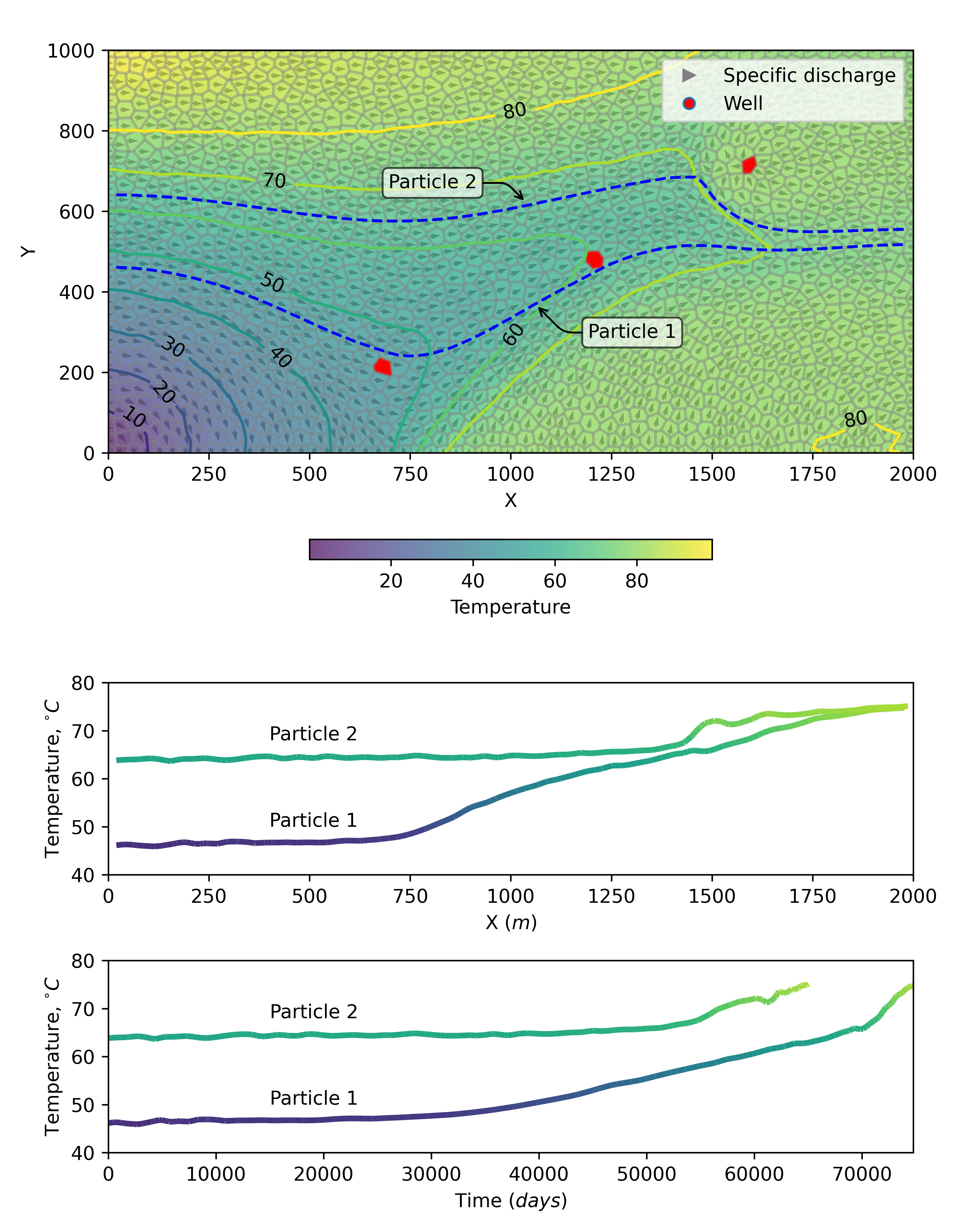
Figure 73.1 (Top) Model grid color-filled with the steady-state temperature field and specific discharge arrows. Dashed blue lines show the paths of particles 1 and 2 and they traverse the simulation domain. (Middle) The x-position of each particle is plotted against its temperature as it traverses the simulation domain. (Bottom) The travel time of each particle is plotted against its temperature as it traverses the simulation domain.
73.3. Jupyter Notebook
The Jupyter notebook used to create the MODFLOW 6 input files for this example and post-process the results is: