19. Flow Diversion
This problem simulates unconfined groundwater flow in an aquifer with a high bottom elevation in the center of the aquifer and groundwater flow around a high bottom elevation.
19.1. Example Description
Model parameters for the example are summarized in Table 19.1. The model consists of a grid of 51 columns, 51 rows, and 1 layer. The discretization is 1.96 \(m\) in the row and column direction for all cells. The top of the aquifer is 25 \(m\) and the bottom elevation of the aquifer ranges from 0 \(m\) at the edges of the domain to 10 \(m\) in the center of the domain (Figure 19.1). A single steady-stress period with a total length of 1 day is simulated.
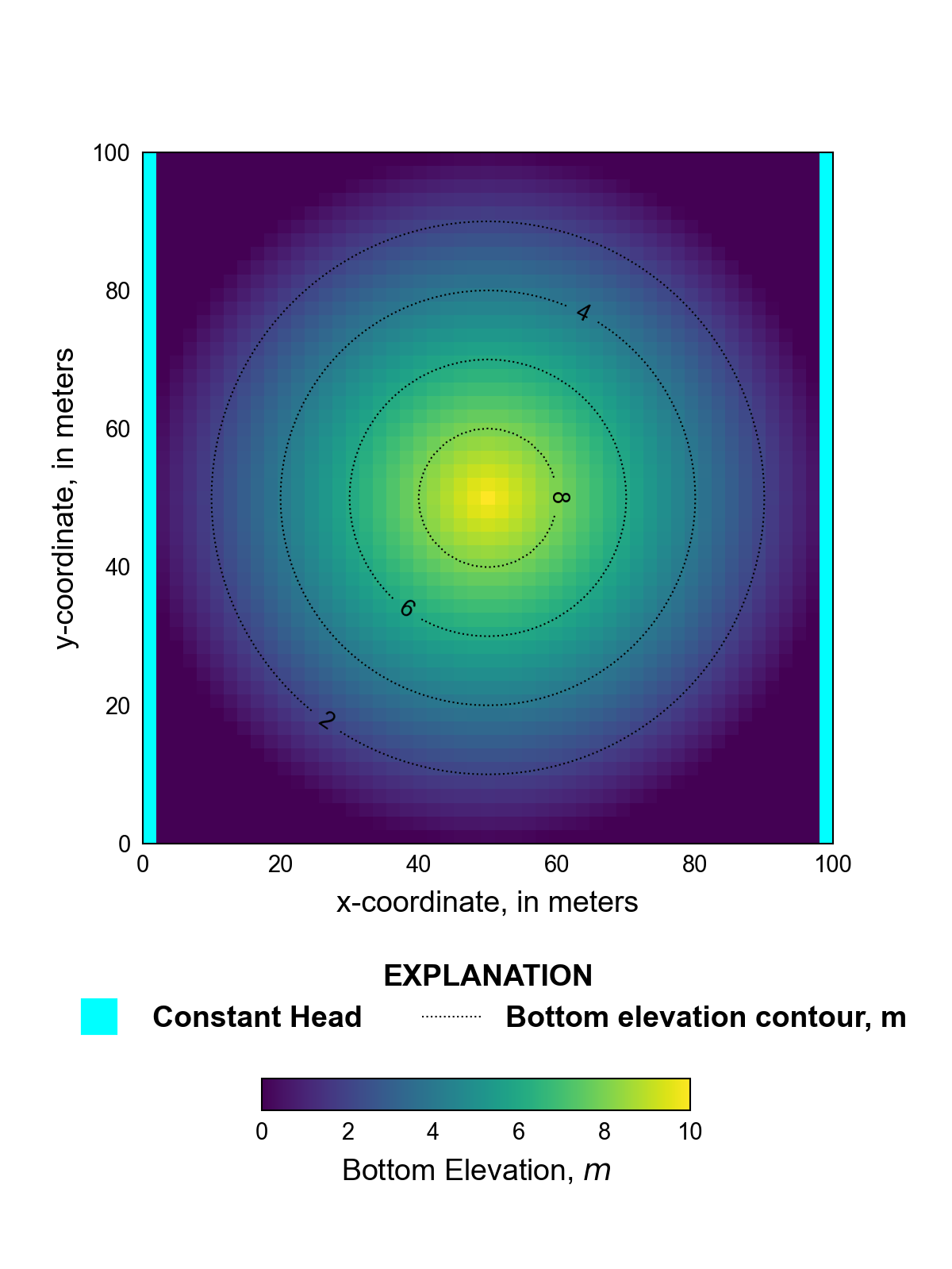
Figure 19.1 Bottom elevation of the flow diversion problem in meters. Bottom elevation are lowest at the edges of the domain and highest in the center of the domain. The location of constant head boundary cells is also shown.
Parameter |
Value |
|---|---|
Number of periods |
1 |
Number of layers |
1 |
Number of rows |
51 |
Number of columns |
51 |
Model length in x-direction (\(m\)) |
100.0 |
Model length in y-direction (\(m\)) |
100.0 |
Top of the model (\(m\)) |
25.0 |
Horizontal hydraulic conductivity (\(m/day\)) |
1.0 |
Constant head in column 1 and starting head (\(m\)) |
7.5 |
Constant head in column 51 (\(m\)) |
2.5 |
A constant horizontal hydraulic conductivity of 1 \(m/day\) was specified in all cells. An initial head of 7.5 \(m\) was specified in all model cells. Constant head boundary cells were specified for all rows in column 1 and 51. A constant head value of 7.5 and 2.5 \(m\) is specified in column 1 and 51, respectively.
19.2. Scenario Results
The flow diversion model was evaluated using the Newton-Raphson Formulation and the Standard Conductance Formulation with rewetting (Table 19.2). A scenario that used a cylindrical obstruction and the Newton-Raphson Formulation was also evaluated.
Scenario |
Scenario Name |
Parameter |
Value |
|---|---|---|---|
1 |
ex-gwf-bump-p01a |
newton |
newton |
2 |
ex-gwf-bump-p01b |
rewet |
True |
wetfct |
1.0 |
||
iwetit |
1 |
||
ihdwet |
0 |
||
wetdry |
2.0 |
||
3 |
ex-gwf-bump-p01c |
newton |
newton |
cylindrical |
True |
19.2.1. Newton-Raphson Formulation
Simulated results using the Newton-Raphson Formulation is shown in Figure 19.2. Newton under-relaxation is used with the Newton-Raphson Formulation to maintain water-levels above the aquifer bottom (Hughes et al., 2017). Cells with bottom elevation ranging from approximately 7.5 to 10 \(m\) are dry and normalized specific discharge vectors show that groundwater is flowing around the dry cells. Note the relatively constant heads of approximately 7.5 \(m\) adjacent to the dry cells. A total of 10.94 \(m^3/day\) is discharged to the constant head cells in column 51.
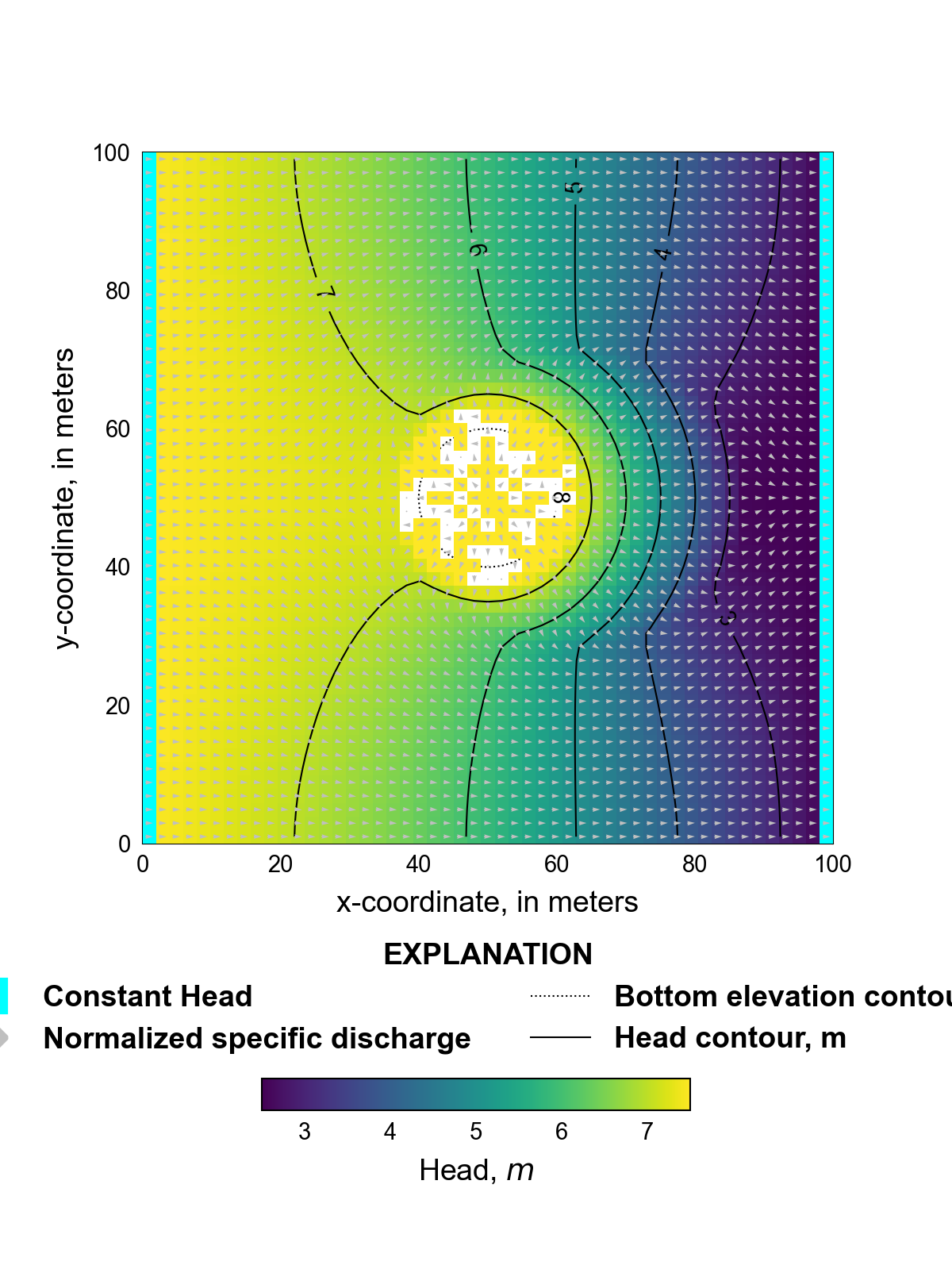
Figure 19.2 Simulated heads and normalized specific discharge vectors for the scenario using the Newton-Raphson Formulation. Bottom elevation contours are shown in areas with dry cells. The location of constant head boundary cells is also shown.
19.2.2. Standard Conductance Formulation with rewetting
Rewetting parameters specified in the Node Property Flow Package for this scenario are summarized in Table 19.2. A positive WETDRY parameter value of 2 is used to allow wetting to occur from horizontally adjacent cells. Simulated results using the Standard Conductance Formulation with rewetting is shown in Figure 19.3. Although the rewetting allows the model to converge the area of dry cells is significantly larger than the area of dry cells in the Newton-Raphson Formulation scenario. Furthermore, the increase in the area of dry cells is not symmetric and extends further in areas where there is a significant component of downstream flow. Simulated heads for both scenarios are comparable in areas that are not dry in both scenarios. A total of 10.50 \(m^3/day\) is discharged to the constant head cells in column 51. The slight flow reduction for this scenario is a result of upstream horizontal conductance weighting used with the Newton-Raphson formulation and the slightly reduced total simulated horizontal conductance for the rewetting scenario.
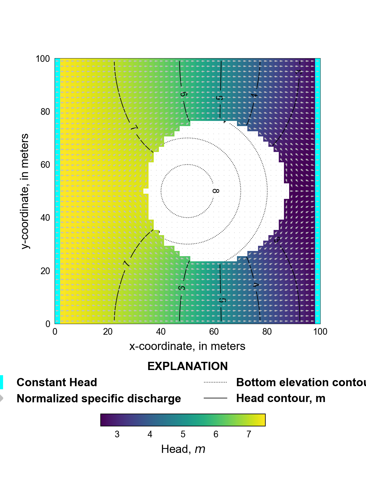
Figure 19.3 Simulated heads and normalized specific discharge vectors for the scenario using the Standard Conductance Formulation with rewetting. Bottom elevation contours are shown in areas with dry cells. The location of constant head boundary cells is also shown.
19.2.3. Newton-Raphson Formulation with a cylindrical obstruction
The model setup for this scenario is identical to the Newton-Raphson Formulation scenario except for the aquifer bottom elevations, which are used to represent the cylindrical obstruction. Aquifer bottom elevations are derived from aquifer bottom elevations shown in Figure 19.1 and are equal to 0 and 20 \(m\) where elevations are less than 7.5 \(m\) and greater than or equal to 7.5 \(m\), respectively. Simulated results using the Newton-Raphson Formulation and a cylindrical obstruction is shown in Figure 19.4. Dry cells are limited to the location of the cylindrical obstruction. Simulated heads for this scenario show the typical characteristics of flow around a cylinder including increased heads on the upstream side of the cylinder and decreased heads on the downstream side of the cylinder. A total of 23.10 \(m^3/day\) is discharged to the constant head cells in column 51, which is more than double to discharge rate in the other scenarios as a result of an increase in total simulated horizontal conductance resulting from bottom elevations equal to 0 \(m\) except in the location of the cylindrical obstruction.
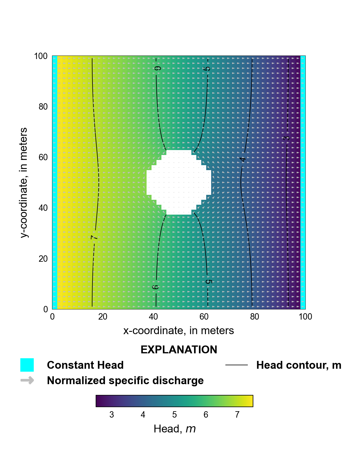
Figure 19.4 Simulated heads and normalized specific discharge vectors for the scenario using the Newton-Raphson Formulation with a cylindrical obstruction. The location of constant head boundary cells is also shown.
19.3. References Cited
Hughes, J. D., Langevin, C. D., & Banta, E. R. (2017). Documentation for the MODFLOW 6 framework. https://doi.org/10.3133/tm6A57
19.4. Jupyter Notebook
The Jupyter notebook used to create the MODFLOW 6 input files for this example and post-process the results is: