44. MT3DMS Problem 8
This example problem originally appeared (Sudicky, 1989) for finding the solution in a hypothetical field-scale example. Among the MT3DMS suite of examples, this is the first one with a heterogeneous hydraulic conductivity field. Defining characteristics that set this problem apart from earlier MT3DMS example problems include a highly irregular flow field and large contrast between longitudinal and transverse dispersivities. (Van der Heijde, 1995) points out that this particular model test potentially troublesome parameter combinations while at the same time testing the ability of a flow and transport code to simulate real-world problems.
44.1. Example description
Using a “deformed quadrilateral” (Zheng & Wang, 1999), the model domain is 250 \(m\) wide by 6.75 \(m\) at at the left boundary and and 5.375 \(m\) at the right boundary. The conceptual model is divided into 27 layers and 50 columns all contained within a single row. For the duration of the simulation, steady flow is maintained by a constant recharge rate of 10 \(cm/yr\), no-flow on the left and bottom boundaries and a constant head of 5.375 \(m\) on the right boundary (Figure 44.1). The simulation uses unconfined conditions to model the water table. Heterogeneity within the aquifer is represented by a fine grained silty sand with a hydraulic conducivity of \(5 \times 10^{-4} cm/sec\) that hosts two lenses of medium-grained sand with a hydraulic conductvity of \(1 \times 10^{-2} cm/sec\) (Table 44.1). The vertical hydraulic conductivity is assumed to equal the horizontal conductivity in both materials.
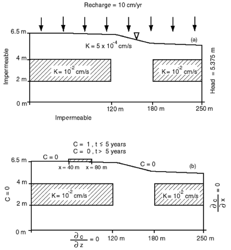
Figure 44.1 MT3DMS test problem 8 configuration showing flow (upper figure) and transport (lower figure) boundary conditions (from (Sudicky, 1989)).
Parameter |
Value |
|---|---|
Number of layers |
27 |
Number of rows |
1 |
Number of columns |
50 |
Column width (\(m\)) |
5.0 |
Row width (\(m\)) |
1.0 |
Layer thickness (\(m\)) |
0.25 |
Top of the model (\(m\)) |
6.75 |
Porosity |
0.35 |
Horiz. hyd. conductivity of fine grain material (\(cm/sec\)) |
5.0e-4 |
Horiz. hyd. conductivity of medium grain material (\(cm/sec\)) |
1.0e-2 |
Applied recharge rate (\(cm/yr\)) |
10.0 |
Longitudinal dispersivity (\(m\)) |
0.5 |
Transverse vertical dispersivity (\(m\)) |
0.005 |
Effective diffusion coefficient (\(cm^2/sec\)) |
1.34e-5 |
Simulation time (\(years\)) |
20.0 |
Boundary conditions within the transport model also are shown in Figure 44.1. A relative concentration of 1.0 is assigned to the recahrge entering the model domain between 40 and 80 \(m\) from the left boundary and 0.0 elsewhere. Mass continues to enter the simulation at the given location for the first five years of the simulation, after which time the source is removed and the model continues to run for an additional 15 years. An initial concentration of 0.0 is specified throughout the model domain. A uniform porosity of 0.35 is assigned to the entire model domain. Additional transport-related parameters are listed in Table 44.1.
44.2. Example results
In order to achieve a close match between MODFLOW 6 and MT3D-USGS, the XT3D solver was activated within MODFLOW 6. Moreover, both solutions use their respective TVD advection schemes. Results are shown after 8, 12, and 20 years (Figure 44.2 - Figure 44.4). In each of the selected years for which results are plotted, model results are similar with a couple of small differences. For example, all plots show the leading edge (as defined by the 0.05 isoconcentration contour) of the MT3DMS-calculated plume ahead of the leading the edge of the MODFLOW 6 plume. Also, the MODFLOW 6 plume is less dispersed compared to the MT3DMS plumes as demonstrated by the presence of higher concentrations (i.e., isoconcentration contours) located at the center of the plume, particularly in years 12 and 20.
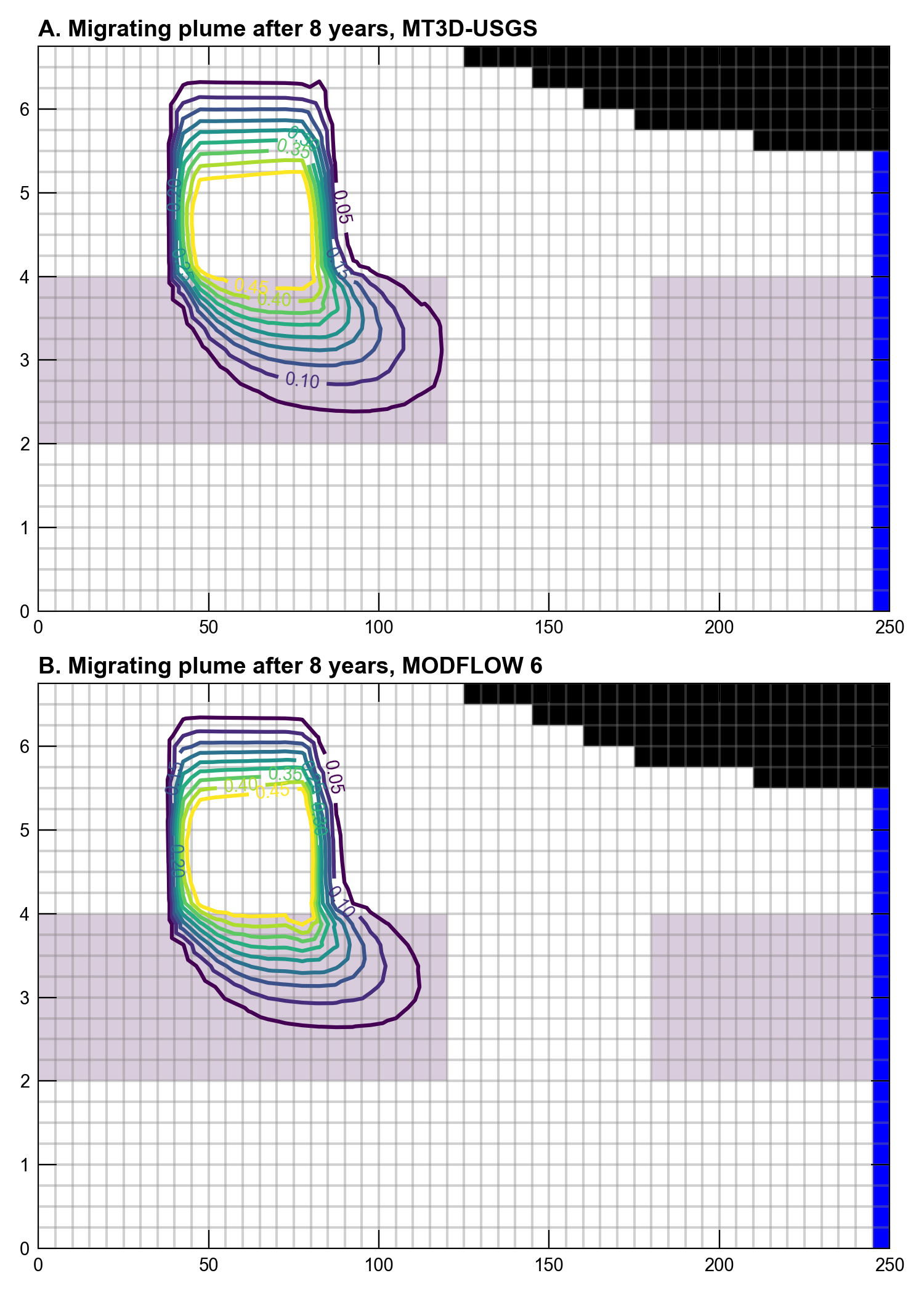
Figure 44.2 Migrating contaminant plume as calculated by (A) MT3D-USGS and (B) MODFLOW 6 after 8 years. The original problem was given in (Sudicky, 1989)
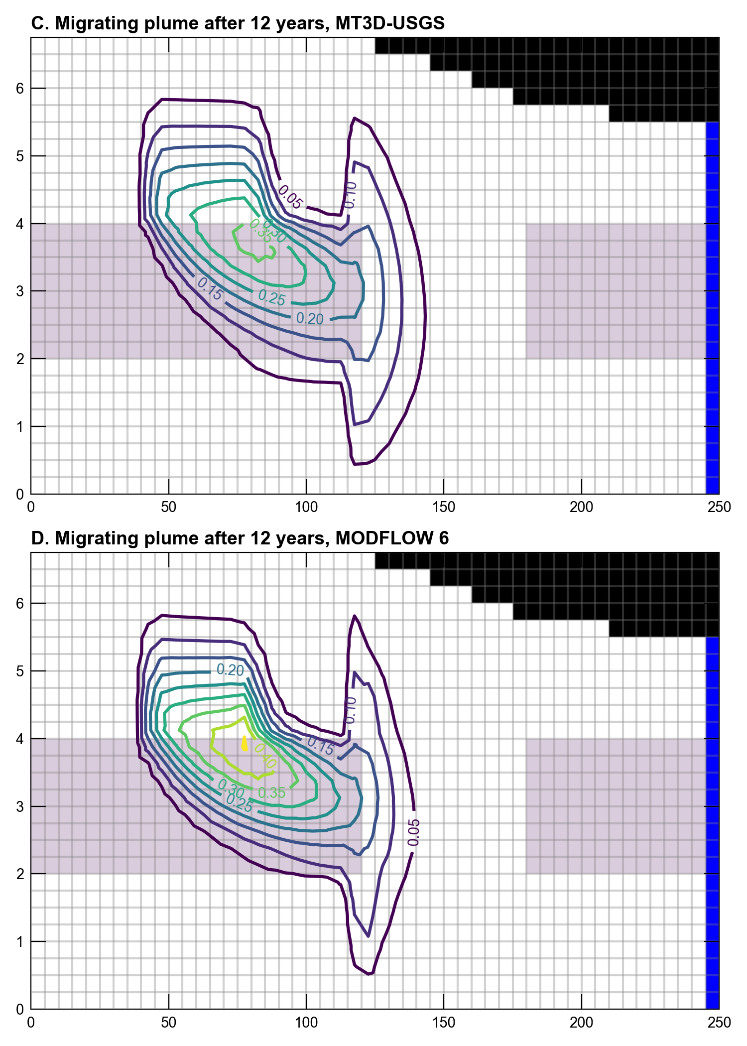
Figure 44.3 Migrating contaminant plume as calculated by (A) MT3D-USGS and (B) MODFLOW 6 after 12 years. The original problem was given in (Sudicky, 1989)
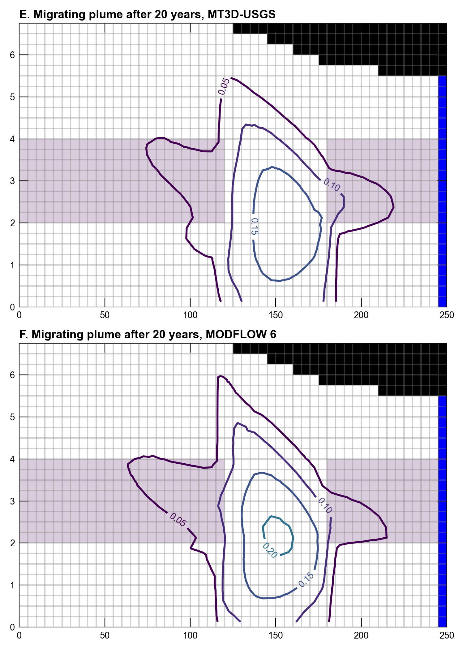
Figure 44.4 Migrating contaminant plume as calculated by (A) MT3D-USGS and (B) MODFLOW 6 after 20 years. The original problem was given in (Sudicky, 1989)
44.3. References Cited
Sudicky, E. (1989). The Laplace transform Galerkin technique–A time‐continuous finite element theory and application to mass transport in groundwater. Water Resources Research, 25(8), 1833–1846. https://doi.org/10.1029/WR025i008p01833
Van der Heijde, P. K. M. (1995). Model testing–A functionality analysis, performance evaluation, and applicability assessment protocol. CRC Press, Lewis Publishers, Boca Raton, FL.
Zheng, C., & Wang, P. P. (1999). MT3DMS—a modular three-dimensional multi-species transport model for simulation of advection, dispersion and chemical reactions of contaminants in groundwater systems; documentation and user’s guide.
44.4. Jupyter Notebook
The Jupyter notebook used to create the MODFLOW 6 input files for this example and post-process the results is: