54. Hecht-Mendez 3D Borehole Heat Exchanger Problem

The models presented in (Hecht-Mendez et al., 2010) apply MT3DMS (Zheng & Wang, 1999) as a heat transport simulator. Both 2-dimensional and 3-dimensional demonstration problems are presented that explore the use of a “borehole heat exchanger” (BHE), a “closed” geothermal system that uses a heat pump for cycling water and anti-freeze fluids in pipes for mining heat from an aquifer (Diao et al., 2004). Figure 54.1 depicts the kind of system modeled in this example.

Among the examples presented in (Hecht-Mendez et al., 2010), this work recreates the 3D example that simulates heat exchange between a BHE and the aquifer it is placed in. Among the suite of examples included in the MODFLOW6-examples.git repo, this is the first one demonstrating the suitability of the GWT model within MODFLOW 6 for simulating saturated zone heat transport. To verify the applicability of MODFLOW 66 as a groundwater heat transport simulator, we compare the MODFLOW 6 solution to established analytical solutions. The analytical solutions are described in more detail below.

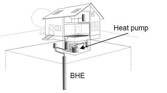
Figure 54.1 Example of a closed ground source heat pump extracting heat beneath a private residence, from (Hecht-Mendez, 2008).

54.1. Example description

Through appropriate substitution of heat-related transport terms into the groundwater solute transport equation, MODFLOW 6(as is the case with MT3DMS and MT3D-USGS) may be used as a heat simulator for the saturated zone by observing that the heat transport equation,

(54.1)\[\theta \rho_w C_w \frac{\partial T}{\partial t} + \left( 1 - \theta \right) \rho_s C_s \frac{\partial T_s}{\partial t} = div \left( \left( k_{T_m} + \theta \rho_w C_w \alpha_h \upsilon_a \right) grad T\right) - div \left( \theta \rho_w C_w \upsilon_a T \right) + q_h,\]

has a similar form as the groundwater solute transport equation,

(54.2)\[\left[ 1 + \frac{\rho_b K_d}{\theta} \right] \theta \frac{\partial C}{\partial t} = div \left[ \theta \left( D_m + \alpha \upsilon_a \right) grad C \right] - div \left( \upsilon_a \theta C \right) + q_s C_s - \lambda \theta C,\]

Originally, (Hecht-Mendez et al., 2010) included three sub-scenarios for the 3D test model. The first sub-scenario used a Peclet number of 0, indicating no velocity and therefore explored a purely conductive environment. Owing to the fact that (Hecht-Mendez et al., 2010) did not publish results for this particular sub-scenario and because a 3D analytical solution for a purely conductive problem is not available, neither is this sub-scenario explored here. The two remaining sub-scenarios investigate the effect of groundwater velocity on the heat profile down-gradient of the BHE. To accomplish this goal, Peclet numbers of 1.0 and 10.0 are explored. A Peclet number of 1.0 indicates an approximate balance between convective (i.e., advective) and conductive heat transport. Meanwhile, a Peclet number of 10.0 represents a convection-dominated transport environment. The parameters used in each of the two scenarios presented are listed in Table 54.1.

Table 54.1 Scenario parameters for example ex-gwt-hecht-mendez.

Scenario	Scenario Name	Parameter	Value
1	ex-gwt-hecht-mendez-a	peclet (\(unitless\))	0.0
		gradient (\(m/m\))	0.0
		seepagevelocity (\(m/s\))	0.0
		constantheadright (\(m\))	14
2	ex-gwt-hecht-mendez-b	peclet (\(unitless\))	1.0
		gradient (\(m/m\))	0.00012
		seepagevelocity (\(m/s\))	3.7e-06
		constantheadright (\(m\))	13.964
3	ex-gwt-hecht-mendez-c	peclet (\(unitless\))	10.0
		gradient (\(m/m\))	0.0012
		seepagevelocity (\(m/s\))	3.7e-05
		constantheadright (\(m\))	13.64

The model grid consists of 83 row, 247 columns, and 13 layers. The flow model solves a steady, confined, uniform flow field moving from left to right, as shown in Figure 54.2. No flow boundaries exist along the north, south, top, and bottom planes of the model domain. The velocity of the groundwater is varied in each of the two modeled scenarios (recall that scenario A is omitted) by varying the fixed head along the east (right) edge of the simulation domain. Cell lengths and widths vary across the model domain, beginning with 0.5 x 0.5 \(m\) grid cells along the perimeter of the model domain, the grid cell resolution is refined to 0.1 x 0.1 \(m\) in the vicinity of the BHE. All layers are set to an equal thickness of 1 \(m\). Additional flow related parameter values are listed in Table 54.2.

Table 54.2 Model parameters for example ex-gwt-hecht-mendez.

Parameter	Value
Number of layers	13
Number of rows	83
Number of columns	247
Column width (\(m\))	varies
Row width (\(m\))	varies
Simulation width (\(m\))	200
Simulation length (\(m\))	300
Layer thickness (\(m\))	1.0
Top of the model (\(m\))	13.0
Saturated thickness (\(m\))	13.0
Horizontal hydraulic conductivity(\(m/s\))	8.0e-3
Vertical hydraulic conductivity(\(m/s\))	8.0e-3
Initial temperature of aquifer (\(K\))	285.15
Porosity	0.26
Longitudinal dispersivity (\(m\))	0.50
Ratio of horizontal transverse dispersivity to longitudinal dispersivity	0.1
Ratio of vertical transverse dispersivity to longitudinal dispersivity	0.1
Aquifer bulk density (\(kg/m^3\))	1961.0
Distribution coefficient (\(m^3/kg\))	2.103e-4
Simulation time (\(seconds\)) (= 150 days)	12960000.0

Because the model is 3D, vertical heat transfer among the layers is considered. The BHE is vertically centered within the model grid, located in layers 6, 7, and 8 and is represented by a constant mass loading boundary condition. A negative mass (i.e., heat) loading rate of -60 \(W/m\) is constant throughout the simulation period and acts as a heat sink within the aquifer. Justification for the selected heat removal rate is given in (Hecht-Mendez et al., 2010). Initially, the entire model domain starts out with a constant temperature of 285.15 \(^{\circ}K\) (12 \(^{\circ}C\)). Additionally, groundwater enters the west boundary of the model at 285.15 \(^{\circ}K\) and leaves at the calculated temperature of the groundwater along the east boundary. Heat exchange does not occur with the no-flow boundaries to facilitate comparison with analytical solutions.

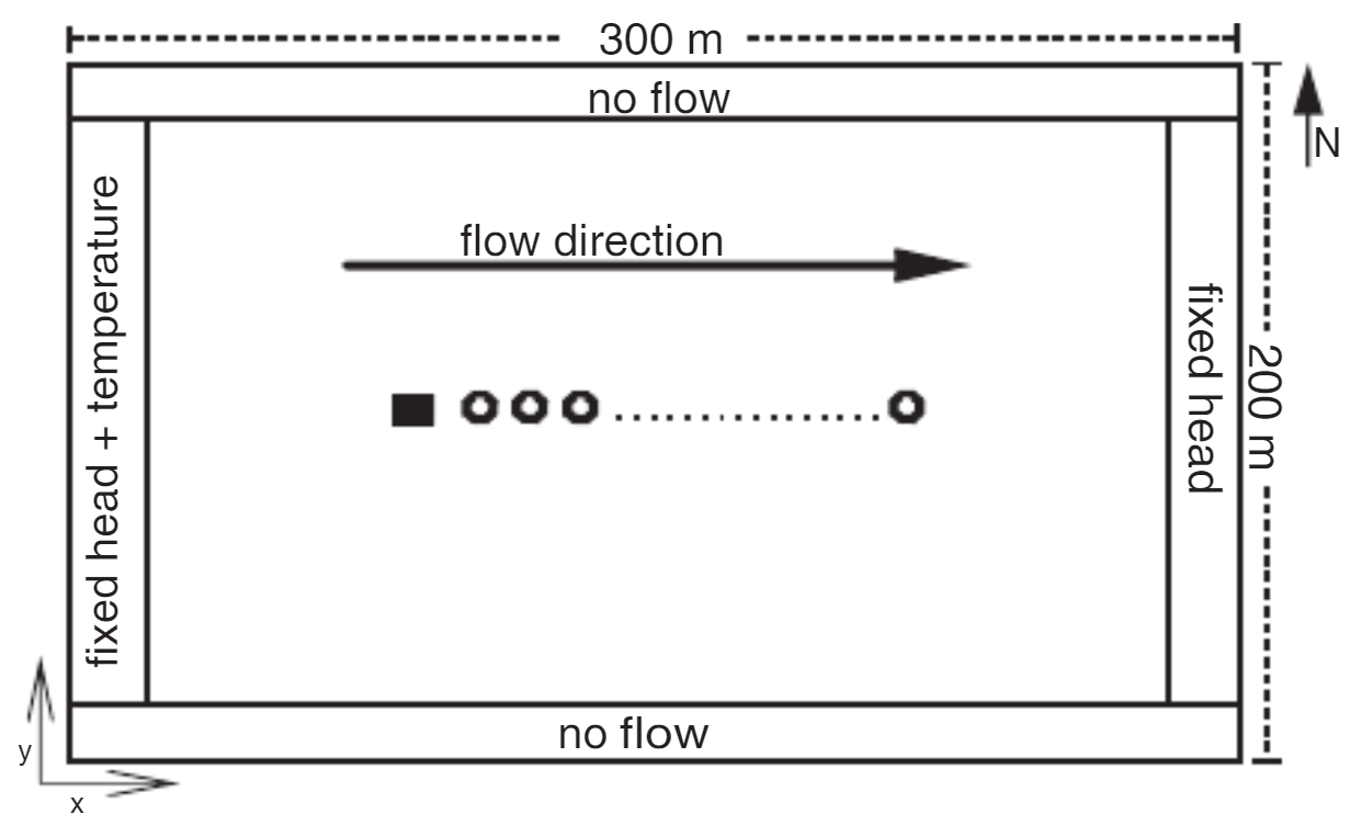
Figure 54.2 Model setup, from (Hecht-Mendez et al., 2010).

54.2. Analytical solutions

For each of the two scenarios simulated here, two points in time are compared to analytical solutions: 10 and 150 days from the start of the simulation representing transient and steady-state conditions. Although simulated results continue to change after 150 days, the magnitude of the change is relatively minor. Thus, 150 days was selected as “close enough” in order to help keep total simulation times to a minimum for obtaining the steady-state solution. Owing to numerical dispersion concerns, the total variation diminishing (TVD) schemes is activated in MODFLOW 6.

The analytical solution for a 3D planar source (or sink) is given in (Domenico & Robbins, 1985) as,

(54.3)\[T \left( x, y, z, t \right) = \frac{T_o}{8} \cdot erfc \left[ \frac{Rx - \upsilon_a t}{2 \sqrt{D_x R t}} \right] \cdot \Bigg\{ erf \left[ \frac{ \left( y + \frac{Y}{2} \right)}{2 \sqrt{D_y \frac{x}{v_a}}} \right] - erf \left[ \frac{ \left( y - \frac{Y}{2} \right)}{2 \sqrt{D_y \frac{x}{v_a}}} \right] \Bigg\} \cdot \Bigg\{ erf \left[ \frac{ \left( z + \frac{Z}{2} \right)}{2 \sqrt{D_z \frac{x}{v_a}}} \right] - erf \left[ \frac{ \left( z - \frac{Z}{2} \right)}{2 \sqrt{D_z \frac{x}{v_a}}} \right] \Bigg\},\]

Y and Z are the dimensions of the sink; \(D_x\), \(D_y\), and \(D_z\) are the dispersion coefficients for dispersivities in the x, y, and z directions, corresponding to \(\alpha_x\), \(\alpha_y\), and \(\alpha_z\); and \(T_o\) is the starting temperature where the BHE is located and is given by,

(54.4)\[T_o = \frac{F}{\upsilon_a \theta \rho_w C_w},\]

where F is the energy extraction per area of the source (\(W/m^2\)). Along the centerline of the plume, depicted in Figure 54.3, the analytical solution under transient conditions reduces to the following,

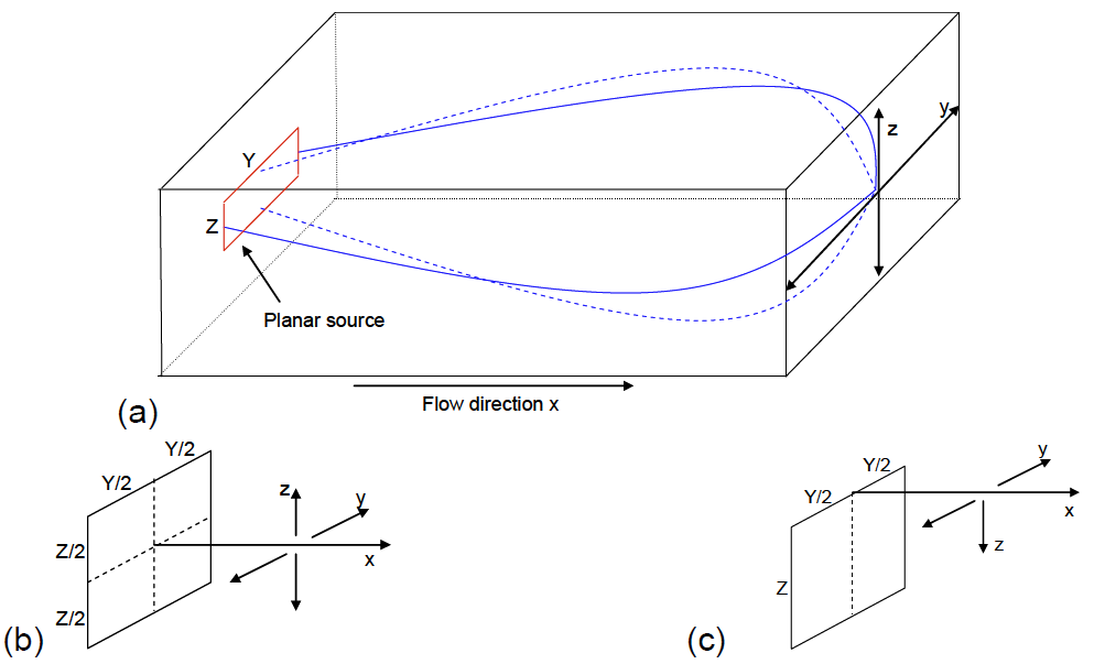
Figure 54.3 (A) Depiction of a heat plume spreading down gradient of a planar source (or sink) for which (Domenico & Robbins, 1985) gives an analytical solution for (B) two spreading directions in both y and z and finally (C) two spreading directions in y and one spreading direction in z, from (Hecht-Mendez, 2008).

(54.5)\[T \left( x, t \right) = \frac{T_o}{2} \cdot erfc \left[ \frac{Rx - \upsilon_a t}{2 \sqrt{D_x R t}} \right] \cdot erf \left[ \frac{ Y }{4 \sqrt{D_y \frac{x}{v_a}}} \right] \cdot erf \left[ \frac{ Z }{4 \sqrt{D_z \frac{x}{v_a}}} \right],\]

For steady-state conditions, the complementary error function (\(erfc\)) term may be neglected while the \(\frac {T_o}{2}\) term reduces to \(T_o\), leaving,

(54.6)\[T \left( x \right) = T_o erf \left[ \frac{ Y }{4 \sqrt{D_y \frac{x}{v_a}}} \right] \cdot erf \left[ \frac{ Z }{4 \sqrt{D_z \frac{x}{v_a}}} \right],\]

Model results are compared to these analytical solutions.

54.3. Example results

Simulated temperature profiles downstream of the BHE are compared to steady-state and transient (10 days after the start of the simulation) analytical solutions in Figure 54.4 (Peclet = 1.0) and Figure 54.5 (Peclet = 10.0). In each scenario, simulated results compare well to the expected (i.e., analytical) temperature profiles, with some undersimulation of the temperature down gradient of the BHE shown in Figure 54.4 (Peclet number equal to 1.0). Discrepancies between the simulated and analytical results are smaller in the scenario with a Pectlet number of 10.0. Moreover, under highly convective flow regimes, the transient solution is approximately equal to the steady state solution after 10 days, as shown in Figure 54.5. These results confirm that MODFLOW 6 may be used as a heat transport simulator in the saturated zone.

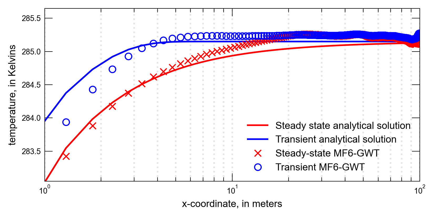
Figure 54.4 MODFLOW 6 simulated temperatures are compared to analytical solutions in a steady flow model with a Peclet number equal to 1.0. For this scenario, thermal transport is roughly split between convective and conductive processes. Temperature profiles are calculated along the centerline down gradient of a planar heat sink as shown in Figure 54.3

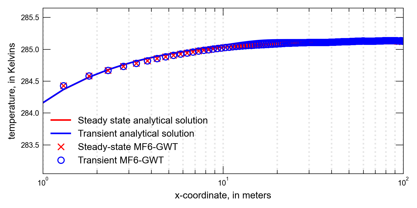
Figure 54.5 MODFLOW 6 simulated temperatures are compared to analytical solutions in a steady flow model with a Peclet number equal to 10.0. For this scenario, thermal transport is dominated by convective transport. Temperature profiles are calculated along the centerline down gradient of a planar heat sink as shown in Figure 54.3

54.4. References Cited

Diao, N., Li, Q., & Fang, Z. (2004). Heat transfer in ground heat exchangers with groundwater advection. International Journal of Thermal Sciences, 43(12), 1203–1211. https://doi.org/10.1016/j.ijthermalsci.2004.04.009

Domenico, P. A., & Robbins, G. A. (1985). A new method of contaminant plume analysis. Groundwater, 23(4), 476–485. https://doi.org/10.1111/j.1745-6584.1985.tb01497.x

Hecht-Mendez, J. (2008). Implementation and verification of the USGS solute transport code MT3DMS for groundwater heat transport modeling. Retrieved from https://www.hechtm.de/onewebmedia/Thesis_with_erratum.pdf

Hecht-Mendez, J., Molina-Giraldo, N., Blum, P. D., & Bayer, P. (2010). Evaluating MT3DMS for heat transport simulation of closed geothermal systems. Groundwater, 48(5), 741–756. https://doi.org/10.1111/j.1745-6584.2010.00678.x

Zheng, C., & Wang, P. P. (1999). MT3DMS—a modular three-dimensional multi-species transport model for simulation of advection, dispersion and chemical reactions of contaminants in groundwater systems; documentation and user’s guide.

54.5. Jupyter Notebook

The Jupyter notebook used to create the MODFLOW 6 input files for this example and post-process the results is:

• ex-gwt-hecht-mendez