20. Circular Island with Triangular Mesh
This example shows how a triangular mesh can be used to simulate a circular island. This is a synthetic example problem that has not been documented elsewhere.
20.1. Example Description
The problem consists of a simple two-layer model representing groundwater flow in a circular island. The island has a radius of 1025 \(m\). The extent of the grid extends out to 1500 \(m\) from the island center. The grid consists of 5240 triangular cells and 2778 vertices per layer. The grid was created using an external mesh generator. Vertices and cell definitions are provided to MODFLOW 6 using the Discretization by Vertices (DISV) Package. There is a single steady-state stress period with a length of 1 day. Model parameters are listed in Table 20.1.
Parameter |
Value |
|---|---|
Number of periods |
1 |
Number of layers |
2 |
Top of the model (\(m\)) |
0.0 |
Layer bottom elevations (\(m\)) |
–20.0, –40.0 |
Starting head (\(m\)) |
0.0 |
Cell conversion type |
0 |
Horizontal hydraulic conductivity (\(m/d\)) |
10.0 |
Vertical hydraulic conductivity (\(m/d\)) |
0.2 |
Recharge rate (\(m/d\)) |
4.0e-3 |
An initial head of 0 \(m\) was specified for the model. The value is not important as the model is steady state.
Recharge is assigned to cells in layer one that are within the 1025 \(m\) radius of the island. Outside the island, general-head boundaries (GHB) are assigned with a stage of zero. GHB locations are shown in cyan in Figure 20.1. Cells not colored in Figure 20.1 are assigned recharge.
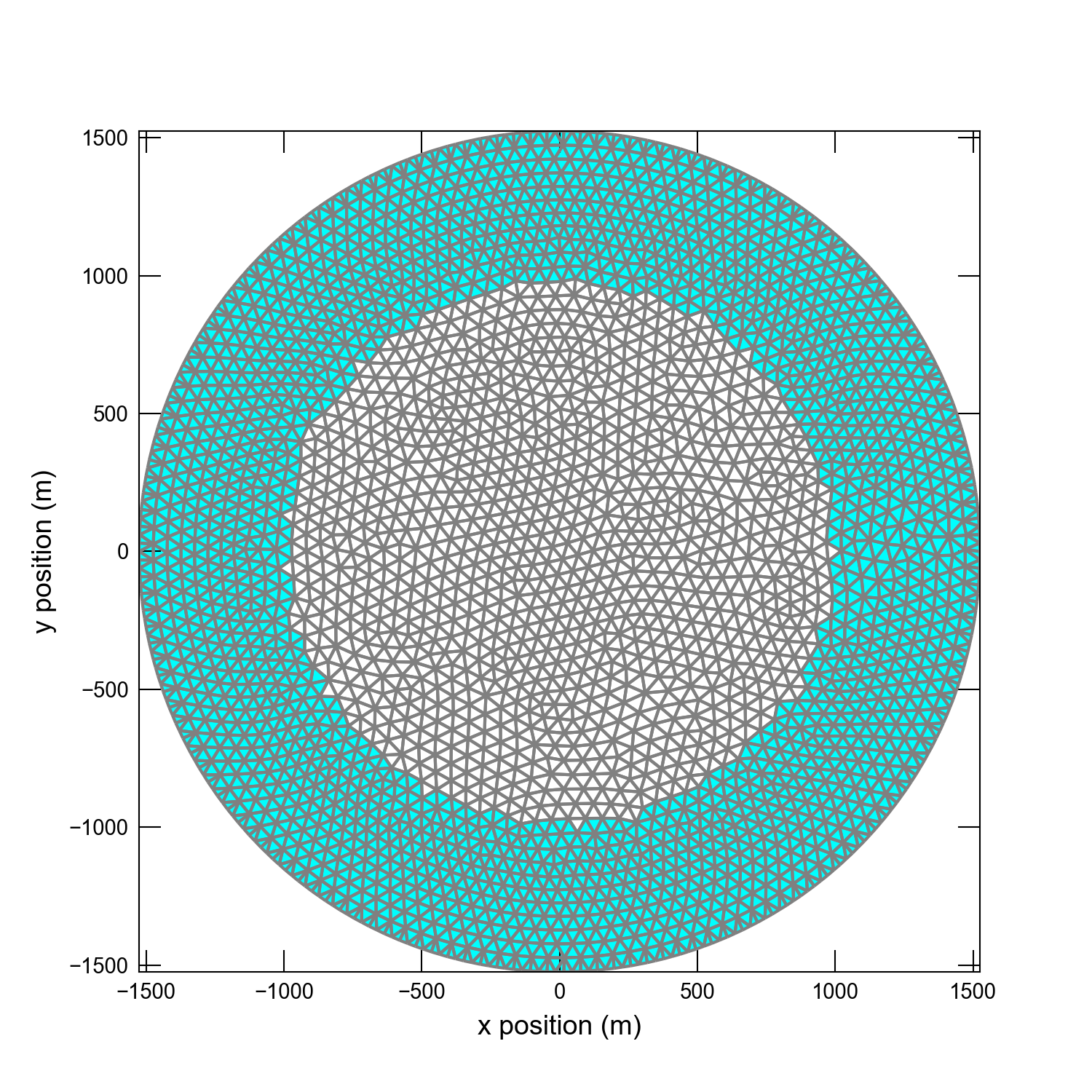
Figure 20.1 Model grid and boundary conditions used for the circular island problem. General-head boundaries are shown in blue, and represent an off-shore boundary condition. Cell not colored represent the island and are assigned groundwater recharge.
20.2. Example Results
Simulated heads for model layers 1 and 2 are shown in Figure 20.2.
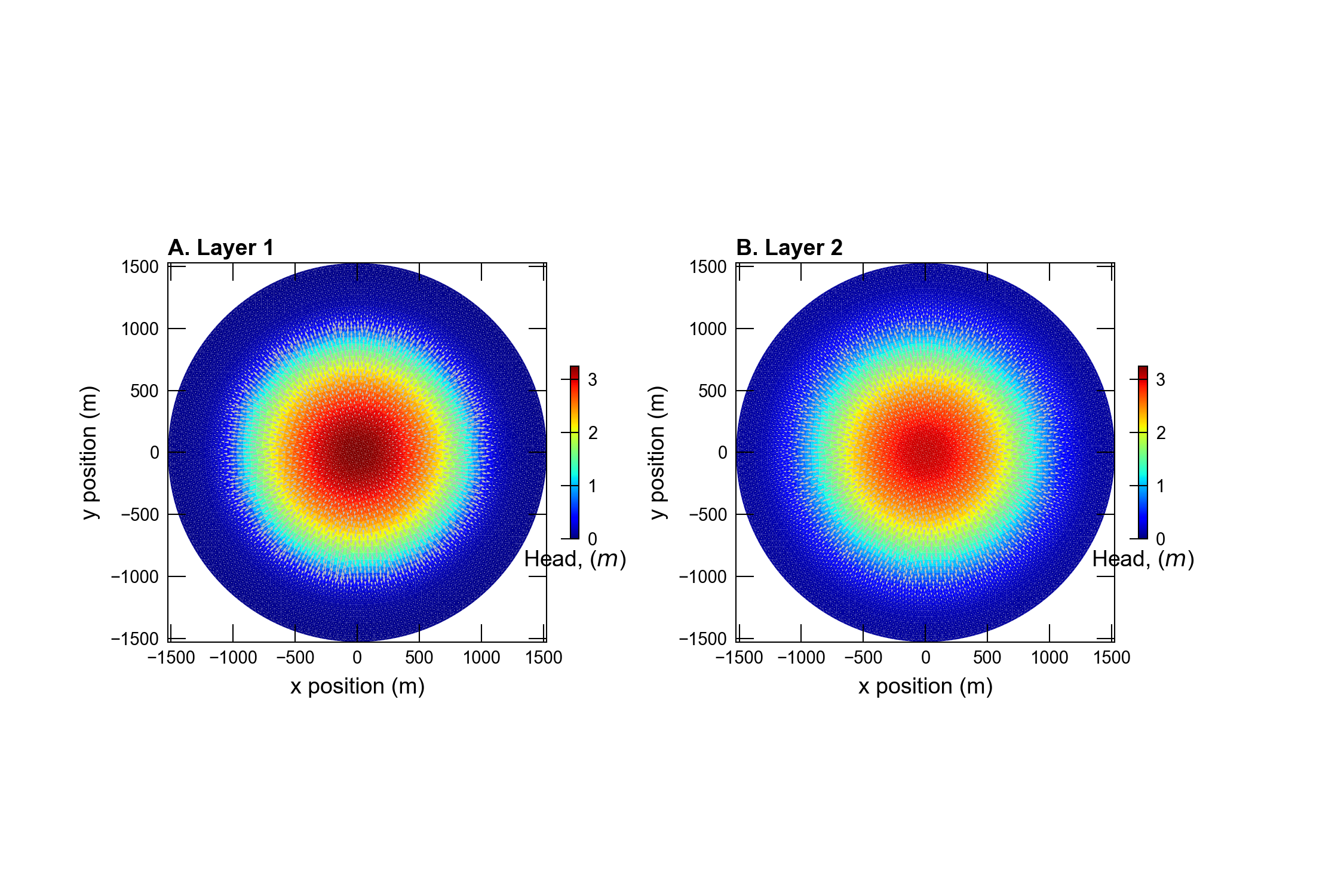
Figure 20.2 Simulated groundwater head in (A) model layer 1 and (B) model layer 2.
20.3. Jupyter Notebook
The Jupyter notebook used to create the MODFLOW 6 input files for this example and post-process the results is: