53. Henry Problem
This problem simulates the classic Henry problem (Henry, 1964) for variable-density groundwater flow and solute transport. The MODFLOW 6 simulations presented here are based on the hydraulic-head formulation for variable-density flow as presented by (Langevin et al., 2020).
53.1. Example Description
Variations on the Henry problem (Henry, 1964) are commonly used as benchmark test problems for variable-density flow and transport codes. The model domain for the Henry problem is 2 \(m\) long by 1 \(m\) tall. In the original version of the problem, for which (Henry, 1964) presented a semianalytical solution, freshwater with a density of 1000 \(kg/m^3\) flows into the domain through the left side at a rate of 5.7024 \(m^3/d\). (Simpson & Clement, 2004) reduced the rate of inflow to 2.851 \(m^3/d\) in their numerical simulations, rendering the flow system less “advective dominant” and effecting “an increase in the relative importance of density-driven processes” (Simpson & Clement, 2004). This modified version of the problem, called the “low-inflow” version here, provides a better benchmark test of density-dependent flow behavior than Henry’s original version. Results from both versions of the problem are presented.
(Henry, 1964) and (Simpson & Clement, 2004) assign the same flow and transport boundary conditions at the right boundary. The boundary condition for flow is a hydrostatic condition based on seawater concentration, 35 \(kg/m^3\), which corresponds to a density of 1024.5 \(kg/m^3\). For transport, the concentration at the right boundary is fixed at seawater concentration. The simulations presented here use a variation in which the right boundary is assigned a mixed boundary condition: water that flows into the model from the right boundary enters at seawater concentration, and water that flows out of the model at the right boundary exits at the groundwater concentration computed for that boundary cell. Use of a mixed boundary condition in the Henry problem was introduced by (Segol et al., 1975), who imposed a Neumann-type condition for transport when water flows out of the model. The mixed boundary condition used here, in which outflow is at the prevailing groundwater concentration, is the condition used for the Henry problem by (Voss, 1984) and (Voss & Souza, 1987). This manner of representing the seawater boundary, which is often used in saltwater intrusion models, allows a freshwater outflow zone to form above the zone of recirculating saltwater.
The freshwater hydraulic conductivity is set to 864 \(m/d\), and the porosity to 0.35 (tab. Table 53.1). Mechanical dispersion is not represented; all mixing occurs solely by molecular diffusion with a diffusion coefficient of 0.57024 \(m^2/d\). The simulation begins with the model domain initially filled with seawater, although the problem can also be simulated with the domain initially filled with freshwater. If the hydraulic head is fixed for the seawater boundary and the mixed boundary condition is used for transport, then it may be necessary to start the simulation with some saltwater in the domain or there may be no seawater inflow. In the simulations presented here, the domain is divided into 40 layers and 80 columns of cells, and a simulation period of 0.5 \(d\) is divided into 500 equally sized time steps of 0.001 \(d\).
Parameter |
Value |
|---|---|
Number of periods |
1 |
Number of time steps |
500 |
Simulation time length (\(d\)) |
0.5 |
Number of layers |
40 |
Number of rows |
1 |
Number of columns |
80 |
Length of system (\(m\)) |
2.0 |
Column width (\(m\)) |
0.025 |
Row width (\(m\)) |
1.0 |
Layer thickness |
0.025 |
Top of the model (\(m\)) |
1.0 |
Hydraulic conductivity (\(m d^{-1}\)) |
864.0 |
Initial concentration (unitless) |
35.0 |
porosity (unitless) |
0.35 |
diffusion coefficient (\(m^2/d\)) |
0.57024 |
53.2. Scenario Results
The original and low-inflow versions of the Henry problem (tab. Table 53.2) were simulated with a mixed boundary condition for concentration in cells along the right boundary. The mixed boundary condition is represented using the General-Head Boundary (GHB) Package, which allows the hydrostatic boundary condition to be effectively imposed at the right edge of the model domain by accounting for the conductance of aquifer material between the cell center and the right edge of the model domain. Conceptually, a seawater reservoir is attached to the edge of each model cell at the right boundary. Flow into the model domain enters at the concentration of seawater, and flow out of the model domain exists at the concentration computed in the corresponding boundary cell. Figure 53.1 shows contours of concentration (relative seawater concentrations of 0.01, 0.1, 0.5, 0.9, and 0.99) at the end of the 0.5 \(d\) simulation period for the classic Henry problem. Figure 53.2 shows results from the low-inflow version of the Henry problem. These same simulations were reported by (Langevin et al., 2020) and were shown to be in good agreement with results from SEAWAT simulations.
Scenario |
Scenario Name |
Parameter |
Value |
|---|---|---|---|
1 |
ex-gwt-henry-a |
inflow (\(m^3/d\)) |
5.7024 |
2 |
ex-gwt-henry-b |
inflow (\(m^3/d\)) |
2.851 |
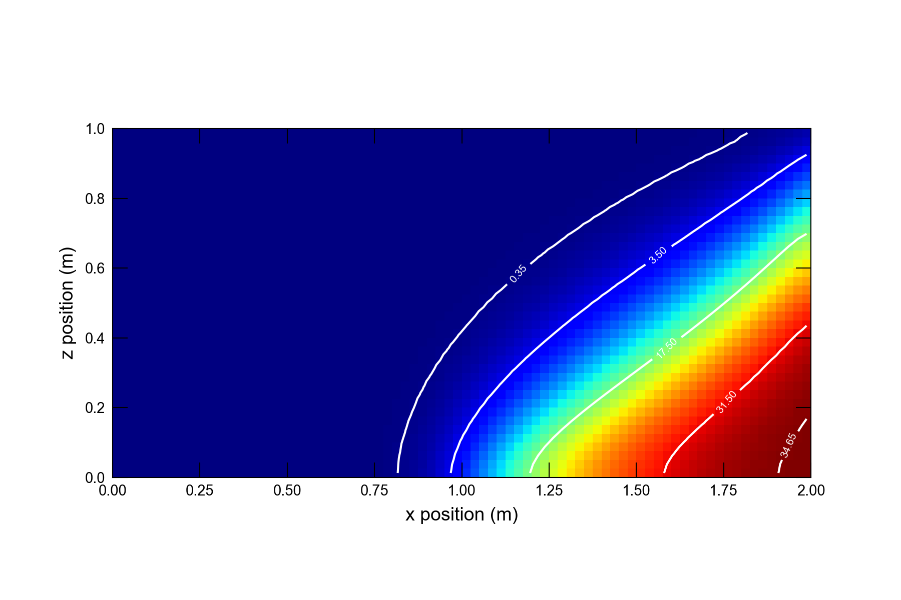
Figure 53.1 Simulation results for the classic Henry problem.
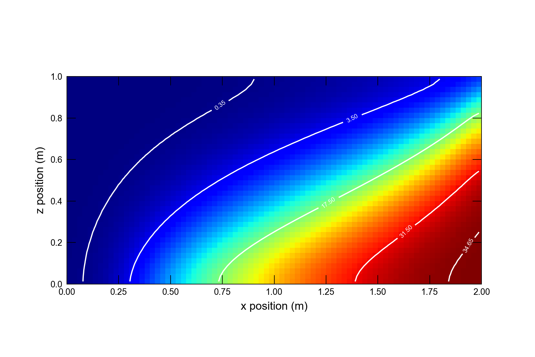
Figure 53.2 Simulation results for the low-inflow version of the Henry problem.
53.3. References Cited
Henry, H. R. (1964). Effects of dispersion on salt encroachment in coastal aquifers.
Langevin, C. D., Panday, S., & Provost, A. M. (2020). Hydraulic-head formulation for density-dependent flow and transport. Groundwater, 58(3), 349–362. https://doi.org/10.1111/gwat.12967
Segol, G., Pinder, G. F., & Gray, W. G. (1975). A Galerkin-finite element technique for calculating the transient position of the saltwater front. Water Resources Research, 11(2), 343–347. https://doi.org/10.1029/WR011i002p00343
Simpson, M. J., & Clement, T. P. (2004). Improving the worthiness of the Henry problem as a benchmark for density-dependent groundwater flow models. Water Resources Research, 40(W01504), 1152–1173. https://doi.org/10.1029/2003WR002199
Voss, C. I. (1984). SUTRA—a finite-element simulation model for saturated-unsaturated fluid-density-dependent ground-water flow with energy transport or chemically-reactive single-species solute transport.
Voss, C. I., & Souza, W. R. (1987). Variable density flow and solute transport simulation of regional aquifers containing a narrow freshwater-saltwater transition zone. Water Resources Research, 23(10), 1851–1866. https://doi.org/10.1029/WR023i010p01851
53.4. Jupyter Notebook
The Jupyter notebook used to create the MODFLOW 6 input files for this example and post-process the results is: