62. Radial Heat Transport
A dedicated heat transport model referred to as the groundwater energy transport (GWE) model was released with version 6.5.0 of MODFLOW 6. Previously, to simulate groundwater heat transport in MODFLOW 6, a user could use the groundwater solute transport model, commonly referred to as simply groundwater transport (without specifying “solute” transport), to mimic heat transport by using its input parameters as surrogates for heat transport parameters (Langevin et al., 2008, 2022; Ma & Zheng, 2010). Now, with GWE, users may specify native heat transport parameter values in the appropriate GWE package.
62.1. Example description
This example demonstrates use of the GWE model. This demonstration compares simulated results from a GWE model to an analytical solution that was published in (Al-Khoury et al., 2020). Both the groundwater flow (GWF) and GWE models employ a DISV grid type (Langevin et al., 2017) with the numerical grid setup in a radial manner (Figure 62.1). The grid geometry facilitates outward propagation of heat from a borehole heat exchanger (BHE) (Hecht-Mendez et al., 2010) located in the center of the radially-symetric model grid (Figure 62.1). Groundwater flow moves from left to right. In this way, the model simulates heat flow in a convective and conductive heat transport environment moving past a cylindrical heat source.
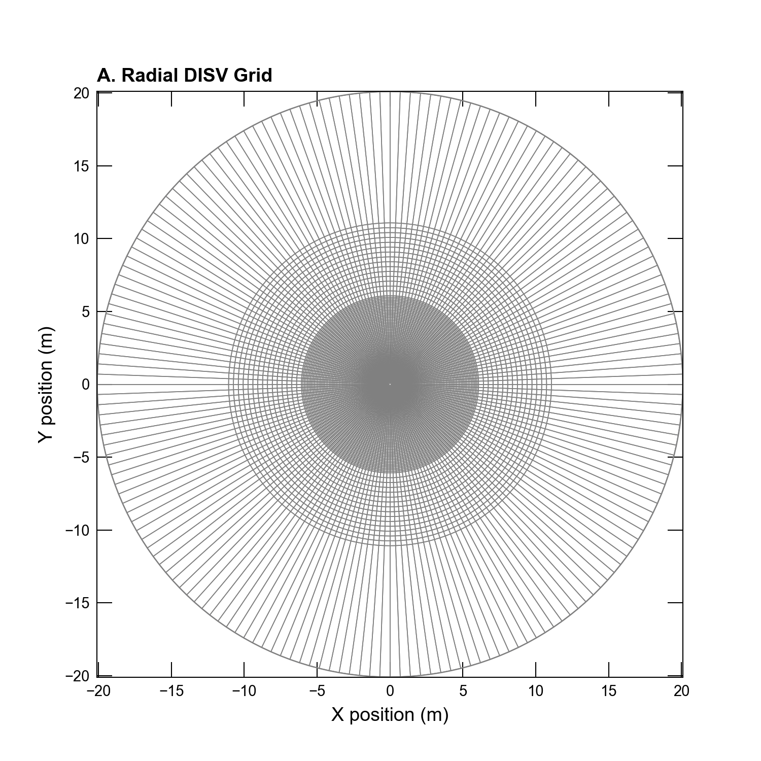
Figure 62.1 Configuration of the DISV model grid used in the radial transport problem. Model grid originally published in (Al-Khoury et al., 2020). Please refer to Figure 62.2 for a zoomed-in view of the model grid in the vicinity of the BHE.
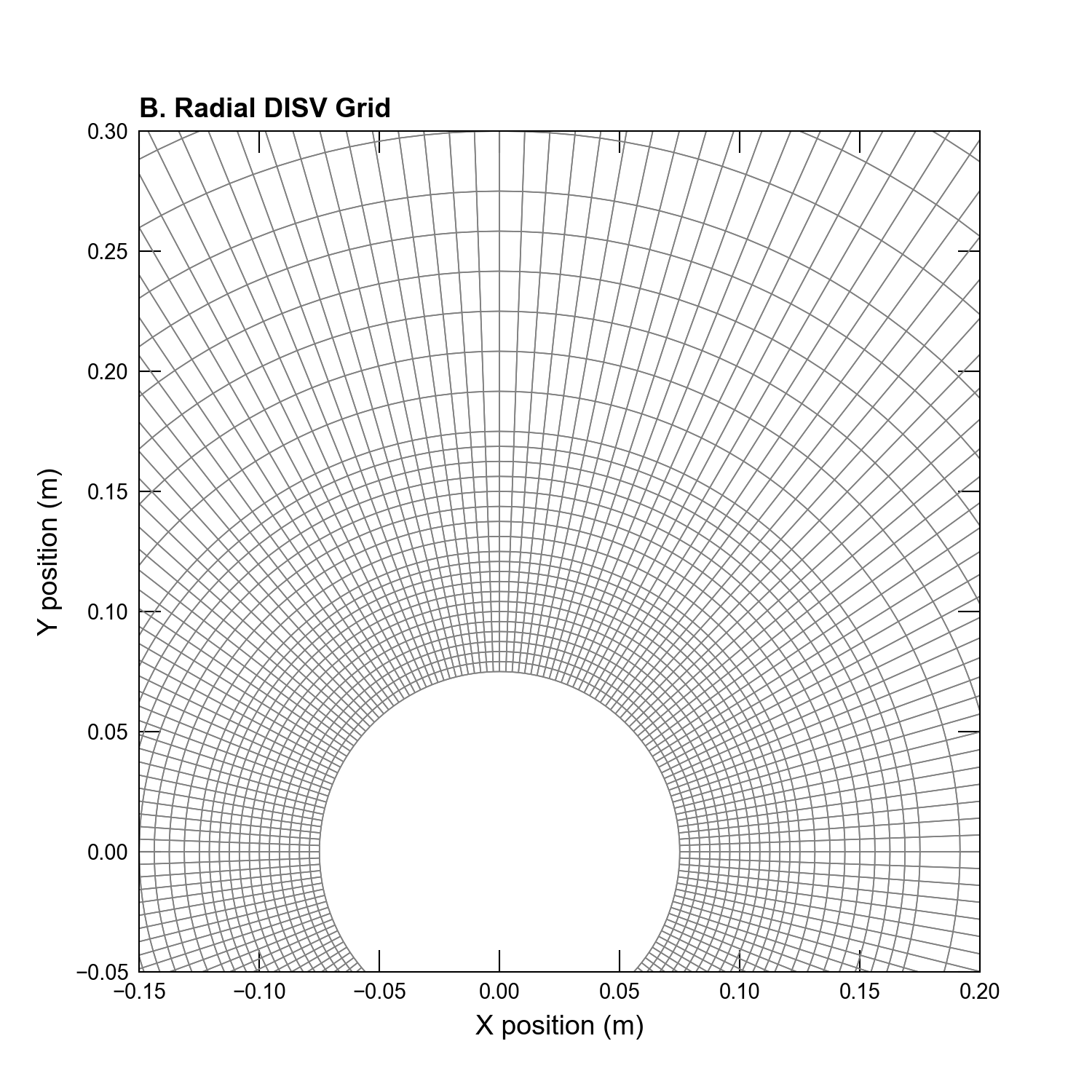
Figure 62.2 A zoomed-in view showing the refined discretization in close proximity to the BHE. Cell dimensions are sub-centimeter scale around the perimeter of the BHE. The radius of the BHE is 7.5 \(cm\).
Constant heads on the left and right sides of the model domain are specified such that the resulting left-to-right groundwater velocity is \(1 \times 10^{-5} \tfrac{m}{s}\) (Figure 62.3). The heat source located in the center of the numerical model is represented using the energy source loading (ESL) package with a known rate of energy input [referred to as a Dirichlet boundary condition in (Al-Khoury et al., 2020)]. The initial temperature throughout the model domain is 0.0 \(^{\circ}C\). Energy is added to the grid cell in the middle of the model domain at a rate of 100 \(\tfrac{W}{m}\). Parameters used for the MODFLOW 6 simulation of the heat transport problem that uses a radially-symmetric grid are shown in Table 62.1.
Parameter |
Value |
|---|---|
Number of periods in flow model (\(-\)) |
1 |
Number of layers (\(-\)) |
1 |
Simulation radius (\(m\)) |
20 |
Horizontal hydraulic conductivity (\(m/d\)) |
1.0 |
Top of the model (\(m\)) |
1.0 |
Bottom of the model (\(m\)) |
0.0 |
Porosity (\(-\)) |
0.2 |
Length of simulation (\(days\)) |
2 |
Initial Temperature (\(^{\circ} C\)) |
0.0 |
Advection solution scheme (\(-\)) |
TVD |
Thermal conductivity of water (\(\frac{W}{m \cdot ^{\circ} C}\)) |
0.56 |
Thermal conductivity of aquifer material (\(\frac{W}{m \cdot ^{\circ} C}\)) |
2.50 |
Density of water (\(kg/m^3\)) |
1000.0 |
Heat capacity of water (\(\frac{J}{kg \cdot ^{\circ} C}\)) |
4180.0 |
Density of dry solid aquifer material (\(kg/m^3\)) |
2650.0 |
Heat capacity of dry solid aquifer material (\(\frac{J}{kg \cdot ^{\circ} C}\)) |
900.0 |
Mechanical dispersion (\(m^2/day\)) |
0.0 |
Transverse dispersivity (\(m^2/day\)) |
0.0 |
Starting head (\(m\)) |
1.0 |
Groundwater seepage velocity 1 (\(m/s\)) |
1.0e-5 |
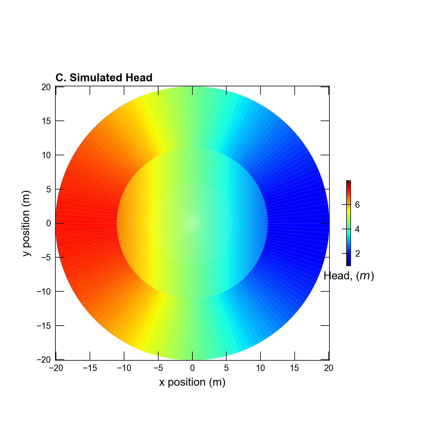
Figure 62.3 A head gradient is established in the outer-most ring of grid cells to drive groundwater flow from left to right. The combination of the groundwater head gradient with the hydraulic conductivity (Table 62.1) results in a groundwater velocity of \(1 \times 10^{-5} \tfrac{m}{s}\).
62.2. Example Results
Results from the GWE model run are compared to a published analytical solution 48 hours after the start of the simulation (Al-Khoury et al., 2020). Isotemperature contours at 1, 2, 3, 4, 6, and 8 \(^{\circ}C\) demonstrate that GWE results compare well with the analytical solution (Figure 62.4).
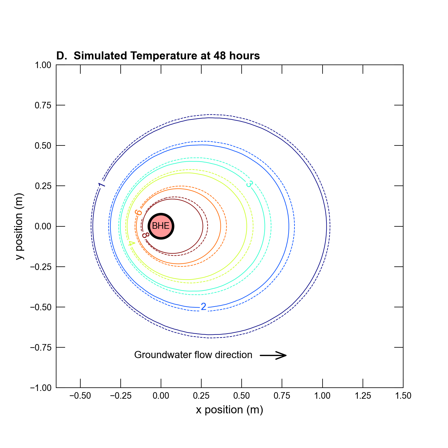
Figure 62.4 Simulation results for the GWE model run compared with an analytical solution.
62.3. References Cited
Al-Khoury, R., BniLam, N., Arzanfudi, M. M., & Saeid, S. (2020). A spectral model for a moving cylindrical heat source in a conductive-convective domain. International Journal of Heat and Mass Transfer, 163, 120517. https://doi.org/10.1016/j.ijheatmasstransfer.2020.120517
Hecht-Mendez, J., Molina-Giraldo, N., Blum, P. D., & Bayer, P. (2010). Evaluating MT3DMS for heat transport simulation of closed geothermal systems. Groundwater, 48(5), 741–756. https://doi.org/10.1111/j.1745-6584.2010.00678.x
Langevin, C. D., Thorne Jr, D. T., Dausman, A. M., Sukop, M. C., & Guo, W. (2008). SEAWAT version 4—a computer program for simulation of multi-species solute and heat transport. U.S. Geological Survey. Retrieved from https://pubs.er.usgs.gov/publication/tm6A22
Langevin, C. D., Hughes, J. D., Provost, A. M., Banta, E. R., Niswonger, R. G., & Panday, S. (2017). MODFLOW 6, the U.S. Geological Survey Modular Hydrologic Model. https://doi.org/10.5066/F76Q1VQV
Langevin, C. D., Provost, A. M., Panday, S., & Hughes, J. D. (2022). Documentation for the MODFLOW 6 groundwater transport (GWT) model. https://doi.org/10.3133/tm6A55
Ma, R., & Zheng, C. (2010). Effects of density and viscosity in modeling heat as a groundwater tracer. Groundwater, 48(3), 380–389. https://doi.org/10.1111/j.1745-6584.2009.00660.x
62.4. Jupyter Notebook
The Jupyter notebook used to create the MODFLOW 6 input files for this example and post-process the results is: