This page was generated from
ex-gwt-synthetic-valley.py.
It's also available as a notebook.
Synthetic Valley Problem
This problem is described in Hughes and others (2023).
Initial setup
Import dependencies, define the example name and workspace, read settings from environment variables, and define some general utilities.
[1]:
from pathlib import Path
from pprint import pformat

import flopy
import flopy.plot.styles as styles
import git
import matplotlib.gridspec as gridspec
import matplotlib.pyplot as plt
import matplotlib.ticker as mticker
import numpy as np
import pooch
import shapely
from flopy.discretization import VertexGrid
from flopy.utils.triangle import Triangle
from flopy.utils.voronoi import VoronoiGrid
from matplotlib import colors
from modflow_devtools.misc import get_env, timed
from shapely.geometry import LineString, Polygon

# Settings from environment variables
write = get_env("WRITE", True)
run = get_env("RUN", True)
plot = get_env("PLOT", True)
plot_show = get_env("PLOT_SHOW", True)
plot_save = get_env("PLOT_SAVE", True)

# Groundwater 2023 utilities

geometries = {
    "sv_boundary": """0.0 0.0
    0.0 20000.0
    12500.0 20000.0
    12500.0 0.0""",
    "sv_river": """4250.0 8750.0
    4250.0 0.0""",
    "sv_river_box": """3500.0 0.0
    3500.0 9500.0
    5000.0 9500.0
    5000.0 0.0""",
    "sv_wells": """7250. 17250.
    7750. 2750.
    2750 3750.""",
    "sv_lake": """1500. 18500.
    3500. 18500.
    3500. 15500.
    4000. 15500.
    4000. 14500.
    4500. 14500.
    4500. 12000.
    2500. 12000.
    2500. 12500.
    2000. 12500.
    2000. 14000.
    1500. 14000.
    1500. 15000.
    1000. 15000.
    1000. 18000.
    1500. 18000.""",
}


def string2geom(geostring, conversion=None):
    if conversion is None:
        multiplier = 1.0
    else:
        multiplier = float(conversion)
    res = []
    for line in geostring.split("\n"):
        line = line.strip()
        line = line.split(" ")
        x = float(line[0]) * multiplier
        y = float(line[1]) * multiplier
        res.append((x, y))
    return res


def densify_geometry(line, step, keep_internal_nodes=True):
    xy = []  # list of tuple of coordinates
    lines_strings = []
    if keep_internal_nodes:
        for idx in range(1, len(line)):
            lines_strings.append(shapely.geometry.LineString(line[idx - 1 : idx + 1]))
    else:
        lines_strings = [shapely.geometry.LineString(line)]

    for line_string in lines_strings:
        length_m = line_string.length  # get the length
        for distance in np.arange(0, length_m + step, step):
            point = line_string.interpolate(distance)
            xy_tuple = (point.x, point.y)
            if xy_tuple not in xy:
                xy.append(xy_tuple)
        # make sure the end point is in xy
        if keep_internal_nodes:
            xy_tuple = line_string.coords[-1]
            if xy_tuple not in xy:
                xy.append(xy_tuple)

    return xy


def circle_function(center=(0, 0), radius=1.0, dtheta=10.0):
    angles = np.arange(0.0, 360.0, dtheta) * np.pi / 180.0
    xpts = center[0] + np.cos(angles) * radius
    ypts = center[1] + np.sin(angles) * radius
    return np.array([(x, y) for x, y in zip(xpts, ypts)])


# Example name and workspace paths. If this example is running
# in the git repository, use the folder structure described in
# the README. Otherwise just use the current working directory.
sim_name = "ex-gwt-synthetic-valley"
try:
    root = Path(git.Repo(".", search_parent_directories=True).working_dir)
except:
    root = None
workspace = root / "examples" if root else Path.cwd()
figs_path = root / "figures" if root else Path.cwd()
data_path = Path(f"../data/{sim_name}")
data_path = data_path if data_path.is_dir() else Path.cwd()

# Conversion factors
ft2m = 1.0 / 3.28081
ft3tom3 = 1.0 * ft2m * ft2m * ft2m
ftpd2cmpy = 1000.0 * 365.25 * ft2m
mpd2cmpy = 100.0 * 365.25
mpd2inpy = 12.0 * 365.25 * 3.28081
Model setup
Define functions to build models, write input files, and run the simulation.
[2]:
# Model units
length_units = "meters"
time_units = "days"

# Model parameters
pertim = 10957.5  # Simulation length ($d$)
ntransport_steps = 60  # Number of transport time steps
nlay = 6  # Number of layers
rainfall = 0.0025  # Rainfall ($m/d$)
evaporation = 0.0019  # Potential evaporation ($m/d$)
sfr_length_conversion = 1.0  # SFR package length unit conversion
sfr_time_conversion = 86400.0  # SFR package time conversion
sfr_width = 3.048  # Stream width ($m$)
sfr_bedthick = 0.3048  # Stream bed thickness ($m$)
sfr_mann = 0.030  # Stream Manning's roughness coefficient
lake_bedleak = 0.0013  # Lake bed leakance ($1/d$)
lak_length_conversion = 1.0  # LAK package length unit conversion
lak_time_conversion = 86400.0  # LAK package time conversion
drn_kv = 0.03048  # Drain vertical hydraulic conductivity ($m/d$)
drn_bed_thickness = 0.3048  # Drain bed thickness ($m$)
drn_depth = 0.3048  # Drain linear scaling depth ($m$)
alpha_l = 75.0  # Longitudinal dispersivity ($m$)
alpha_th = 7.5  # Transverse horizontal dispersivity ($m$)
porosity = 0.2  # Aquifer porosity (unitless)
confining_porosity = 0.4  # Confining unit porosity (unitless)
[3]:
# voronoi grid properties
maximum_area = 150.0 * 150.0
well_dv = 300.0
boundary_refinement = 100.0
river_refinement = 25.0
lake_refinement = 30.0
max_boundary_area = boundary_refinement * boundary_refinement
max_river_area = river_refinement * river_refinement
max_lake_area = lake_refinement * lake_refinement

boundary_polygon = string2geom(geometries["sv_boundary"], conversion=ft2m)
bp = np.array(boundary_polygon)
bp_densify = np.array(densify_geometry(bp, boundary_refinement))

river_polyline = string2geom(geometries["sv_river"], conversion=ft2m)
sg = np.array(river_polyline)
sg_densify = np.array(densify_geometry(sg, river_refinement))

river_boundary = string2geom(geometries["sv_river_box"], conversion=ft2m)
rb = np.array(river_boundary)
rb_densify = np.array(densify_geometry(rb, river_refinement))

lake_polygon = string2geom(geometries["sv_lake"], conversion=ft2m)
lake_plot = string2geom(geometries["sv_lake"], conversion=ft2m)
lake_plot += [lake_plot[0]]
lake_plot = np.array(lake_plot)
lp = np.array(lake_polygon)
lp_densify = np.array(densify_geometry(lp, lake_refinement))

well_points = string2geom(geometries["sv_wells"], conversion=ft2m)
wp = np.array(well_points)
[4]:
# create the voronoi grid
temp_path = Path("temp/triangle_data")
temp_path.mkdir(parents=True, exist_ok=True)
tri = Triangle(angle=30, nodes=sg_densify, model_ws=temp_path)
tri.add_polygon(bp_densify)
tri.add_polygon(rb_densify)
tri.add_polygon(lp_densify)
tri.add_region((10, 10), attribute=10, maximum_area=max_boundary_area)
tri.add_region((3050.0, 3050.0), attribute=10, maximum_area=max_boundary_area)
tri.add_region((900.0, 4600.0), attribute=11, maximum_area=max_lake_area)
tri.add_region((1200.0, 150.0), attribute=10, maximum_area=max_river_area)
for idx, w in enumerate(wp):
    center = (w[0], w[1])
    tri.add_polygon(circle_function(center=center, radius=100.0))
    tri.add_region(center, attribute=idx, maximum_area=500.0)
tri.build(verbose=False)
vor = VoronoiGrid(tri)
[5]:
# create a vertex grid from the voronoi grid
gridprops = vor.get_gridprops_vertexgrid()
idomain_vor = np.ones((1, vor.ncpl), dtype=int)
voronoi_grid = VertexGrid(**gridprops, nlay=1, idomain=idomain_vor)
[6]:
# load raster data files
fname = "k_aq_SI.tif"
fpath = pooch.retrieve(
    url=f"https://github.com/MODFLOW-ORG/modflow6-examples/raw/master/data/{sim_name}/{fname}",
    fname=fname,
    path=data_path,
    known_hash="md5:d233e5c393ab6c029c63860d73818856",
)
kaq = flopy.utils.Raster.load(fpath)

fname = "k_clay_SI.tif"
fpath = pooch.retrieve(
    url=f"https://github.com/MODFLOW-ORG/modflow6-examples/raw/master/data/{sim_name}/{fname}",
    fname=fname,
    path=data_path,
    known_hash="md5:a08999c37f42b35884468e4ef896d5f9",
)
kclay = flopy.utils.Raster.load(fpath)

fname = "top_SI.tif"
fpath = pooch.retrieve(
    url=f"https://github.com/MODFLOW-ORG/modflow6-examples/raw/master/data/{sim_name}/{fname}",
    fname=fname,
    path=data_path,
    known_hash="md5:781155bdcc2b9914e1cad6b10de0e9c7",
)
top_base = flopy.utils.Raster.load(fpath)

fname = "bottom_SI.tif"
fpath = pooch.retrieve(
    url=f"https://github.com/MODFLOW-ORG/modflow6-examples/raw/master/data/{sim_name}/{fname}",
    fname=fname,
    path=data_path,
    known_hash="md5:00b4a39fbf5180e65c0367cdb6f15c93",
)
bot = flopy.utils.Raster.load(fpath)

fname = "lake_location_SI.tif"
fpath = pooch.retrieve(
    url=f"https://github.com/MODFLOW-ORG/modflow6-examples/raw/master/data/{sim_name}/{fname}",
    fname=fname,
    path=data_path,
    known_hash="md5:38600d6f0eef7c033ede278252dc6343",
)
lake_location = flopy.utils.Raster.load(fpath)
Downloading data from 'https://github.com/MODFLOW-ORG/modflow6-examples/raw/master/data/ex-gwt-synthetic-valley/k_aq_SI.tif' to file '/home/runner/work/modflow6-examples/modflow6-examples/modflow6-examples/.doc/_notebooks/k_aq_SI.tif'.
Downloading data from 'https://github.com/MODFLOW-ORG/modflow6-examples/raw/master/data/ex-gwt-synthetic-valley/k_clay_SI.tif' to file '/home/runner/work/modflow6-examples/modflow6-examples/modflow6-examples/.doc/_notebooks/k_clay_SI.tif'.
Downloading data from 'https://github.com/MODFLOW-ORG/modflow6-examples/raw/master/data/ex-gwt-synthetic-valley/top_SI.tif' to file '/home/runner/work/modflow6-examples/modflow6-examples/modflow6-examples/.doc/_notebooks/top_SI.tif'.
Downloading data from 'https://github.com/MODFLOW-ORG/modflow6-examples/raw/master/data/ex-gwt-synthetic-valley/bottom_SI.tif' to file '/home/runner/work/modflow6-examples/modflow6-examples/modflow6-examples/.doc/_notebooks/bottom_SI.tif'.
Downloading data from 'https://github.com/MODFLOW-ORG/modflow6-examples/raw/master/data/ex-gwt-synthetic-valley/lake_location_SI.tif' to file '/home/runner/work/modflow6-examples/modflow6-examples/modflow6-examples/.doc/_notebooks/lake_location_SI.tif'.
[7]:
# a few variables for plotting
xcv, ycv = voronoi_grid.xcellcenters, voronoi_grid.ycellcenters
x0 = x1 = sg[:, 0].min()
y0, y1 = sg[:, 1].max(), sg[:, 1].min()
top_range = (0, 20)
top_levels = np.arange(0, 25, 5)
head_range = (-1, 5)
head_levels = np.arange(1, head_range[1] + 1, 1)
extent = voronoi_grid.extent
[8]:
# intersect the rasters with the vertex grid
top_vg = top_base.resample_to_grid(
    voronoi_grid, band=top_base.bands[0], method="linear", extrapolate_edges=True
)
bot_vg = bot.resample_to_grid(
    voronoi_grid, band=bot.bands[0], method="linear", extrapolate_edges=True
)
lake_cells_vg = lake_location.resample_to_grid(
    voronoi_grid, band=lake_location.bands[0], method="nearest", extrapolate_edges=True
)
kaq_vg = kaq.resample_to_grid(
    voronoi_grid, band=kaq.bands[0], method="nearest", extrapolate_edges=True
)
kclay_vg = kclay.resample_to_grid(voronoi_grid, band=kclay.bands[0], method="nearest")
[9]:
# create confining unit location map
kclay_loc_vg = np.zeros(kclay_vg.shape, dtype=int)
kclay_loc_vg[kclay_vg < 60.0] = 1
idomain_2 = np.ones(kclay_vg.shape, dtype=int)
idomain_2[kclay_loc_vg == 0] = -1

# set the porosity based on the clay location
porosity_2 = np.full(kclay_vg.shape, porosity, dtype=float)
porosity_2[kclay_loc_vg == 1] = confining_porosity
[10]:
# set the bottom of each layer
bot_l2 = np.full(bot_vg.shape, -51.0 * ft2m, dtype=float)
bot_l3 = np.full(bot_vg.shape, -100.0 * ft2m, dtype=float)
bot_l4 = bot_vg + 0.5 * (bot_l3 - bot_vg)
# set the bottom of the 3rd layer in areas where the confining unit exists
bot_l2[idomain_2 == -1] = -50.0 * ft2m
# create a list with bottom data
botm = [-5.0 * ft2m, -50.0 * ft2m, bot_l2, -100.0 * ft2m, bot_l4, bot_vg]
[11]:
# create a modelgrid for the lake
lake_grid_top = np.full((vor.ncpl), 50.0, dtype=float)
lake_vg_grid = flopy.discretization.VertexGrid(
    **gridprops,
    nlay=1,
    idomain=idomain_vor,
    top=lake_grid_top,
    botm=top_vg.reshape(1, vor.ncpl),
)
[12]:
# intersect stream features with the grid
ixs = flopy.utils.GridIntersect(voronoi_grid)
sg_result = ixs.intersect(
    LineString(sg_densify), sort_by_cellid=False, geo_dataframe=False
)

# build sfr package datasets
sfr_plt_array = np.zeros(voronoi_grid.ncpl, dtype=int)
sfr_nodes = np.arange(0, sg_result.shape[0])
gwf_nodes = sg_result["cellids"][::-1]
sfr_lengths = sg_result["lengths"][::-1]
total_cond = 1800000.0 * ft3tom3
sfr_hk = total_cond * sfr_bedthick / (sfr_width * sfr_lengths.sum())
b0, b1 = -0.3 * ft2m, -2.05 * ft2m
sfr_slope = -0.0002
cum_dist = np.zeros(sfr_nodes.shape, dtype=float)
cum_dist[0] = 0.5 * sfr_lengths[0]
for idx in range(1, sfr_nodes.shape[0]):
    cum_dist[idx] = cum_dist[idx - 1] + 0.5 * (sfr_lengths[idx - 1] + sfr_lengths[idx])
sfr_bot = b0 + sfr_slope * cum_dist
sfr_conn = []
for idx, node in enumerate(sfr_nodes):
    iconn = [node]
    if idx > 0:
        iconn.append(sfr_nodes[idx - 1])
    if idx < sfr_nodes.shape[0] - 1:
        iconn.append(-sfr_nodes[idx + 1])
    sfr_conn.append(iconn)

# <rno> <cellid(ncelldim)> <rlen> <rwid> <rgrd> <rtp> <rbth> <rhk> <man> <ncon> <ustrf> <ndv>
sfrpak_data = []
for idx, (cellid, rlen, rtp) in enumerate(zip(gwf_nodes, sfr_lengths, sfr_bot)):
    sfr_plt_array[cellid] = 1
    sfrpak_data.append(
        (
            idx,
            (0, cellid),
            rlen,
            sfr_width,
            -sfr_slope,
            rtp,
            sfr_bedthick,
            sfr_hk,
            sfr_mann,
            (len(sfr_conn[idx]) - 1),
            1.0,
            0,
        )
    )
sfr_spd = [(node, "rainfall", rainfall) for node in sfr_nodes] + [
    (node, "evaporation", evaporation) for node in sfr_nodes
]
[13]:
# build lake package datasets
lake_ic = 11.3 * ft2m
idx = np.where(lake_cells_vg == 1.0)

lake_map = np.ones(voronoi_grid.ncpl, dtype=int) * -1
lake_map[idx] = 0

(idomain, lakpak_dict, lak_connections) = flopy.mf6.utils.get_lak_connections(
    voronoi_grid, lake_map, bedleak=lake_bedleak
)

# add concentration to lake data as aux
lakpak_data = [(0, lake_ic, lakpak_dict[0], 1.0)]
lake_spd = [
    (0, "rainfall", rainfall),
    (0, "evaporation", evaporation),
]
[14]:
# build drain package datasets
areas = []
for idx in range(voronoi_grid.ncpl):
    vertices = np.array(voronoi_grid.get_cell_vertices(idx))
    area = Polygon(vertices).area
    areas.append(area)
drn_spd = []
for idx, elev in enumerate(top_vg):
    if lake_cells_vg[idx] > 0:
        cond = drn_kv * areas[idx] / drn_bed_thickness
        drn_spd.append([(0, idx), elev, cond, -drn_depth])
[15]:
# build well package datasets
well_loc = []
for x, y in well_points:
    well_loc.append(voronoi_grid.intersect(x, y))

# first well is Virginia City well site 2
# second well is Reilly well
# third well is Virginia City well site 1
well_boundnames = ["P3", "P1", "P2"]
rates = [-1900.0, -7600.0, -7600.0]
welspd = [
    [nlay - 1, cellid, rates[idx], well_boundnames[idx]]
    for idx, cellid in enumerate(well_loc)
]
Model setup
Define functions to build models, write input files, and run the simulation.
[16]:
def build_mf6gwf(sim_folder):
    print(f"Building mf6gwf model...{sim_folder}")
    name = "flow"
    sim_ws = workspace / sim_folder / "mf6gwf"
    sim = flopy.mf6.MFSimulation(
        sim_name=name,
        sim_ws=sim_ws,
        exe_name="mf6",
        continue_=True,
    )
    tdis = flopy.mf6.ModflowTdis(sim, time_units="days", perioddata=((pertim, 1, 1.0),))
    ims = flopy.mf6.ModflowIms(
        sim,
        print_option="all",
        complexity="simple",
        linear_acceleration="bicgstab",
    )
    gwf = flopy.mf6.ModflowGwf(
        sim,
        modelname=name,
        save_flows=True,
        newtonoptions="NEWTON UNDER_RELAXATION",
    )
    dis = flopy.mf6.ModflowGwfdisv(
        gwf,
        length_units="meters",
        nlay=nlay,
        ncpl=vor.ncpl,
        nvert=vor.nverts,
        top=top_vg,
        botm=botm,
        vertices=vor.get_disv_gridprops()["vertices"],
        cell2d=vor.get_disv_gridprops()["cell2d"],
        idomain=[1, 1, idomain_2, 1, 1, 1],
    )
    ic = flopy.mf6.ModflowGwfic(gwf, strt=11.0)
    npf = flopy.mf6.ModflowGwfnpf(
        gwf,
        xt3doptions=True,
        save_specific_discharge=True,
        save_saturation=True,
        icelltype=[1, 0, 0, 0, 0, 0],
        k=[kaq_vg, kaq_vg, kclay_vg, kaq_vg, kaq_vg, kaq_vg],
        k33=[
            0.25 * kaq_vg,
            0.25 * kaq_vg,
            kclay_vg,
            0.25 * kaq_vg,
            0.25 * kaq_vg,
            0.25 * kaq_vg,
        ],
    )
    rch = flopy.mf6.ModflowGwfrcha(gwf, recharge=rainfall)
    evt = flopy.mf6.ModflowGwfevta(gwf, surface=top_vg, rate=evaporation, depth=1.0)
    wel = flopy.mf6.ModflowGwfwel(gwf, stress_period_data=welspd, boundnames=True)
    drn = flopy.mf6.ModflowGwfdrn(
        gwf,
        auxiliary=["depth"],
        auxdepthname="depth",
        stress_period_data=drn_spd,
    )
    sfr = flopy.mf6.ModflowGwfsfr(
        gwf,
        print_stage=True,
        print_flows=True,
        length_conversion=sfr_length_conversion,
        time_conversion=sfr_time_conversion,
        stage_filerecord=f"{name}.sfr.stage.bin",
        budget_filerecord=f"{name}.sfr.cbc",
        nreaches=len(sfrpak_data),
        packagedata=sfrpak_data,
        connectiondata=sfr_conn,
        perioddata=sfr_spd,
    )
    lak = flopy.mf6.ModflowGwflak(
        gwf,
        pname="LAK-1",
        time_conversion=lak_time_conversion,
        length_conversion=lak_length_conversion,
        auxiliary=["concentration"],
        print_stage=True,
        print_flows=True,
        stage_filerecord=f"{name}.lak.stage.bin",
        budget_filerecord=f"{name}.lak.cbc",
        nlakes=1,
        packagedata=lakpak_data,
        connectiondata=lak_connections,
        perioddata=lake_spd,
    )
    oc = flopy.mf6.ModflowGwfoc(
        gwf,
        head_filerecord=name + ".hds",
        budget_filerecord=name + ".cbc",
        saverecord=[("HEAD", "ALL"), ("BUDGET", "ALL")],
        printrecord=[("BUDGET", "ALL")],
    )
    return sim


def build_mf6gwt(sim_folder):
    print(f"Building mf6gwt model...{sim_folder}")
    name = "trans"
    sim_ws = workspace / sim_folder / "mf6gwt"
    sim = flopy.mf6.MFSimulation(
        sim_name=name,
        sim_ws=sim_ws,
        exe_name="mf6",
        continue_=True,
    )
    tdis = flopy.mf6.ModflowTdis(
        sim, time_units="days", perioddata=((pertim, ntransport_steps, 1.0),)
    )
    ims = flopy.mf6.ModflowIms(
        sim,
        print_option="all",
        complexity="simple",
        linear_acceleration="bicgstab",
    )
    gwt = flopy.mf6.ModflowGwt(sim, modelname=name)
    dis = flopy.mf6.ModflowGwtdisv(
        gwt,
        length_units="meters",
        nlay=nlay,
        ncpl=vor.ncpl,
        nvert=vor.nverts,
        top=top_vg,
        botm=botm,
        vertices=vor.get_disv_gridprops()["vertices"],
        cell2d=vor.get_disv_gridprops()["cell2d"],
        idomain=[1, 1, idomain_2, 1, 1, 1],
    )
    ic = flopy.mf6.ModflowGwtic(gwt, strt=0.0)
    adv = flopy.mf6.ModflowGwtadv(gwt, scheme="tvd")
    dsp = flopy.mf6.ModflowGwtdsp(
        gwt,
        diffc=0.0e-12,
        alh=alpha_l,
        ath1=alpha_th,
    )
    mst = flopy.mf6.ModflowGwtmst(
        gwt,
        porosity=[
            porosity_2,
            porosity,
            porosity_2,
            porosity,
            porosity,
            porosity,
        ],
    )
    pd = [
        ("GWFHEAD", "../mf6gwf/flow.hds", None),
        ("GWFBUDGET", "../mf6gwf/flow.cbc", None),
    ]
    fmi = flopy.mf6.ModflowGwtfmi(gwt, packagedata=pd)
    sourcerecarray = [
        ("LAK-1", "AUX", "CONCENTRATION"),
    ]
    ssm = flopy.mf6.ModflowGwtssm(gwt, sources=sourcerecarray)

    oc = flopy.mf6.ModflowGwtoc(
        gwt,
        concentration_filerecord=f"{name}.ucn",
        saverecord=[("CONCENTRATION", "LAST")],
        printrecord=[("BUDGET", "ALL")],
    )
    return sim


def build_models(sim_name):
    sim_mf6gwf = build_mf6gwf(sim_name)
    sim_mf6gwt = build_mf6gwt(sim_name)
    sim_mf2005 = None  # build_mf2005(sim_name)
    sim_mt3dms = None  # build_mt3dms(sim_name, sim_mf2005)
    return sim_mf6gwf, sim_mf6gwt, sim_mf2005, sim_mt3dms


def write_models(sims, silent=True):
    sim_mf6gwf, sim_mf6gwt, sim_mf2005, sim_mt3dms = sims
    sim_mf6gwf.write_simulation(silent=silent)
    sim_mf6gwt.write_simulation(silent=silent)


@timed
def run_models(sims, silent=True):
    sim_mf6gwf, sim_mf6gwt, sim_mf2005, sim_mt3dms = sims
    success, buff = sim_mf6gwf.run_simulation(silent=silent, report=True)
    assert success, pformat(buff)
    success, buff = sim_mf6gwt.run_simulation(silent=silent, report=True)
    assert success, pformat(buff)
Plotting results
Define functions to plot model results.
[17]:
# Figure properties
two_panel_figsize = (17.15 / 2.541, 0.8333 * 17.15 / 2.541)
one_panel_figsize = (8.25 / 2.541, 13.25 / 2.541)
six_panel_figsize = (17.15 / 2.541, 1.4 * 0.8333 * 17.15 / 2.541)
levels = np.arange(10, 110, 10)
contour_color = "black"
contour_style = "--"
sv_contour_dict = {
"linewidths": 0.5,
"colors": contour_color,
"linestyles": contour_style,
}
sv_contour_dict = {
"linewidths": 0.5,
"colors": contour_color,
"linestyles": contour_style,
}
sv_gwt_contour_dict = {
"linewidths": 0.75,
"colors": contour_color,
"linestyles": contour_style,
}
contour_label_dict = {
"linewidth": 0.5,
"color": contour_color,
"linestyle": contour_style,
}
contour_gwt_label_dict = {
"linewidth": 0.75,
"color": contour_color,
"linestyle": contour_style,
}
clabel_dict = {"inline": True, "fmt": "%1.0f", "fontsize": 6, "inline_spacing": 0.5}
font_dict = {"fontsize": 5, "color": "black"}
grid_dict = {"lw": 0.25, "color": "0.5"}
arrowprops = {
"arrowstyle": "-",
"edgecolor": "red",
"lw": 0.5,
"shrinkA": 0.15,
"shrinkB": 0.15,
}
river_dict = {"color": "blue", "linestyle": "-", "linewidth": 1}
lake_cmap = colors.ListedColormap(["cyan"])
clay_cmap = colors.ListedColormap(["brown"])
def plot_wells(ax=None, ms=None):
if ax is None:
ax = plt.gca()
ax.plot(wp[:, 0], wp[:, 1], "ro", ms=ms)
return ax
def plot_river(ax=None):
if ax is None:
ax = plt.gca()
ax.plot(sg_densify[:, 0], sg_densify[:, 1], **river_dict)
return ax
def plot_lake(ax=None, lw=0.5, color="cyan", marker=None, densify=False):
if ax is None:
ax = plt.gca()
if densify:
arr = lp_densify
else:
arr = lake_plot
ax.plot(arr[:, 0], arr[:, 1], ls="-", color=color, lw=lw, marker=marker)
return ax
def set_ticklabels(
ax,
fmt="{:.1f}",
skip_xticklabels=False,
skip_yticklabels=False,
skip_xlabel=False,
skip_ylabel=False,
xticks=None,
yticks=None,
):
if xticks is None:
labels = [ax.get_xticks().tolist()]
else:
ax.set_xticks(xticks, labels=[str(value) for value in xticks])
labels = [xticks]
if yticks is None:
labels += [ax.get_yticks().tolist()]
else:
ax.set_yticks(yticks, labels=[str(value) for value in yticks])
labels += [yticks]
for idx, label in enumerate(labels):
for jdx, value in enumerate(label):
labels[idx][jdx] = fmt.format(float(value) / 1000.0)
if skip_xticklabels:
ax.set_xticklabels([])
else:
ax.xaxis.set_major_locator(mticker.FixedLocator(ax.get_xticks()))
ax.set_xticklabels(labels[0])
if skip_yticklabels:
ax.set_yticklabels([])
else:
ax.yaxis.set_major_locator(mticker.FixedLocator(ax.get_yticks()))
ax.set_yticklabels(labels[1])
if not skip_xlabel:
ax.set_xlabel("x position (km)")
if not skip_ylabel:
ax.set_ylabel("y position (km)")
def plot_well_labels(ax):
for xy, name in zip(well_points, well_boundnames):
styles.add_annotation(
ax=ax,
text=name,
xy=xy,
xytext=(-15, 10),
bold=False,
textcoords="offset points",
arrowprops=arrowprops,
)
def plot_feature_labels(ax):
styles.add_text(
ax=ax,
text="Blue\nLake",
x=610,
y=5000.0,
transform=False,
bold=False,
ha="center",
va="center",
)
styles.add_text(
ax=ax,
text="Straight River",
x=1425,
y=1500.0,
transform=False,
bold=False,
va="center",
ha="center",
rotation=90,
)
plot_well_labels(ax)
def plot_results(sims, idx):
print("Plotting model results...")
plot_river_mapping(sims, idx)
plot_head_results(sims, idx)
plot_conc_results(sims)
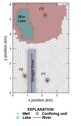
def plot_river_mapping(sims, idx):
print("Plotting river mapping...")
sim_mf6gwf, _, _, _ = sims
sim_ws = Path(sim_mf6gwf.simulation_data.mfpath.get_sim_path())
dv = 100.0 # m
with styles.USGSMap():
fig = plt.figure(figsize=one_panel_figsize, constrained_layout=False)
gs = gridspec.GridSpec(ncols=1, nrows=24, figure=fig)
ax0 = fig.add_subplot(gs[:18])
ax_leg = fig.add_subplot(gs[18:])
ax = ax0
ax.set_aspect("equal", "box")
mm = flopy.plot.PlotMapView(modelgrid=voronoi_grid, ax=ax)
mm.plot_array(kclay_loc_vg, masked_values=[0], cmap=clay_cmap, alpha=0.5)
mm.plot_array(lake_cells_vg, masked_values=[0], cmap=lake_cmap, alpha=0.5)
mm.plot_grid(**grid_dict)
plot_river(ax)
plot_wells(ax, ms=3)
plot_feature_labels(ax)
xticks = np.arange(mm.extent[0], mm.extent[1], 1000.0).tolist()
yticks = np.arange(mm.extent[2], mm.extent[3], 1000.0).tolist()
set_ticklabels(ax, fmt="{:.0f}", xticks=xticks, yticks=yticks)
# legend
ax = ax_leg
xy0 = (-100, -100)
ax.set_ylim(0, 1)
ax.set_axis_off()
# fake data to set up legend
ax.plot(
xy0,
xy0,
lw=0.0,
marker=".",
ms=5,
mfc="red",
mec="none",
mew=0.0,
label="Well",
)
ax.plot(
xy0,
xy0,
lw=0.0,
marker="s",
mfc="cyan",
mec="black",
mew=0.5,
alpha=0.5,
label="Lake",
)
ax.plot(
xy0,
xy0,
lw=0.0,
marker="s",
mfc="brown",
mec="black",
mew=0.5,
alpha=0.5,
label="Confining unit",
)
ax.axhline(xy0[0], **river_dict, label="River")
styles.graph_legend(
ax,
ncol=2,
loc="lower center",
labelspacing=0.1,
columnspacing=0.6,
handletextpad=0.3,
)
if plot_show:
plt.show()
if plot_save:
sim_folder = sim_ws.parent.name
fname = f"{sim_folder}-river-discretization.png"
fig.savefig(figs_path / fname)
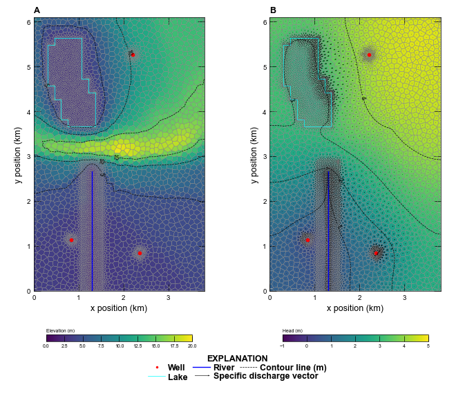
def plot_head_results(sims, idx):
print("Plotting gwf model results...")
sim_mf6gwf, _, _, _ = sims
sim_ws = Path(sim_mf6gwf.simulation_data.mfpath.get_sim_path())
gwf = sim_mf6gwf.flow
xlims = (extent[0], extent[1])
ylims = (extent[2], extent[3])
p2_loc = tuple(welspd[-1][0:2])
p2_z = gwf.modelgrid.zcellcenters[p2_loc]
head = gwf.output.head().get_data().squeeze()
cbc = gwf.output.budget()
spdis = cbc.get_data(text="DATA-SPDIS")[0]
qx, qy, qz = flopy.utils.postprocessing.get_specific_discharge(
spdis, gwf, head=head
)
lake_q = cbc.get_data(text="LAK", full3D=True)[0]
lake_q_dir = np.zeros(lake_q.shape, dtype=int)
lake_q_dir[lake_q < 0.0] = -1
lake_q_dir[lake_q > 0.0] = 1
lake_stage = float(gwf.lak.output.stage().get_data().squeeze())
lake_stage_vg = np.full(vor.ncpl, 1e30, dtype=float)
idx = (lake_stage > top_vg) & (lake_cells_vg > 0)
lake_stage_vg[idx] = lake_stage
with styles.USGSMap():
fig = plt.figure(figsize=two_panel_figsize, constrained_layout=True)
gs = gridspec.GridSpec(ncols=2, nrows=24, figure=fig)
ax0 = fig.add_subplot(gs[:22, 0])
ax1 = fig.add_subplot(gs[:22, 1])
ax2 = fig.add_subplot(gs[22:, :])
xticks = np.arange(extent[0], extent[1], 1000.0).tolist()
yticks = np.arange(extent[2], extent[3], 1000.0).tolist()
for ax in (ax0, ax1):
ax.set_xlim(xlims)
ax.set_xticks(xticks)
ax.set_ylim(ylims)
ax.set_yticks(yticks)
ax.set_aspect("equal", "box")
# topography
ax = ax0
styles.heading(ax=ax, idx=0)
mm = flopy.plot.PlotMapView(model=gwf, ax=ax, extent=voronoi_grid.extent)
cb = mm.plot_array(top_vg, vmin=top_range[0], vmax=top_range[1])
mm.plot_grid(**grid_dict)
plot_wells(ax=ax, ms=3)
plot_river(ax=ax)
plot_lake(ax=ax)
cs = mm.contour_array(top_vg, **sv_contour_dict, levels=top_levels)
ax.clabel(cs, **clabel_dict)
set_ticklabels(ax, fmt="{:.0f}")
# topography colorbar
cbar = plt.colorbar(cb, ax=ax, orientation="horizontal", shrink=0.65)
cbar.ax.tick_params(
labelsize=5, labelcolor="black", color="black", length=6, pad=2
)
cbar.ax.set_title("Elevation (m)", pad=2.5, loc="left", fontdict=font_dict)
# head
ax = ax1
styles.heading(ax=ax, idx=1)
mm = flopy.plot.PlotMapView(model=gwf, ax=ax, extent=voronoi_grid.extent)
cb = mm.plot_array(head, vmin=head_range[0], vmax=head_range[1])
mm.plot_grid(**grid_dict)
q = mm.plot_vector(qx, qy, normalize=False)
qk = plt.quiverkey(
q,
-0.35,
-0.31,
1.0,
label="Specific discharge vector",
labelsep=0.05,
labelpos="E",
labelcolor="black",
fontproperties={"size": 9, "weight": "bold"},
)
plot_wells(ax=ax, ms=3)
plot_river(ax=ax)
plot_lake(ax=ax)
cs = mm.contour_array(head, **sv_contour_dict, levels=head_levels)
ax.clabel(cs, **clabel_dict)
set_ticklabels(ax, fmt="{:.0f}", xticks=xticks, yticks=yticks)
# head colorbar
cbar = plt.colorbar(cb, ax=ax, orientation="horizontal", shrink=0.65)
cbar.ax.tick_params(
labelsize=5, labelcolor="black", color="black", length=6, pad=2
)
cbar.ax.set_title("Head (m)", pad=2.5, loc="left", fontdict=font_dict)
# legend
ax = ax2
xy0 = (-100, -100)
ax.set_xlim(0, 1)
ax.set_ylim(0, 1)
ax.set_axis_off()
# fake data to set up legend
well_patch = ax.plot(
xy0,
xy0,
lw=0.0,
marker=".",
ms=5,
mfc="red",
mec="none",
mew=0.0,
label="Well",
)
lake_patch = ax.axhline(xy0[0], color="cyan", lw=0.5, label="Lake")
river_patch = ax.axhline(xy0[0], **river_dict, label="River")
contour_patch = ax.axhline(
xy0[0], **contour_label_dict, label="Contour line (m)"
)
styles.graph_legend(
ax,
ncol=3,
loc="lower center",
labelspacing=0.1,
columnspacing=0.6,
handletextpad=0.3,
)
if plot_show:
plt.show()
if plot_save:
sim_folder = sim_ws.parent.name
fname = f"{sim_folder}-head.png"
fig.savefig(figs_path / fname)
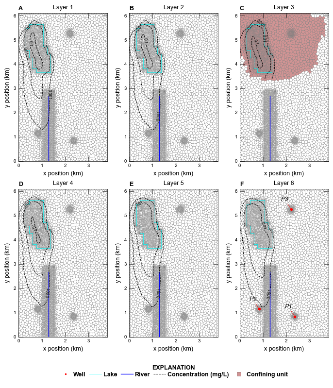
def plot_conc_results(sims):
print("Plotting gwt model results...")
_, sim_mf6gwt, _, _ = sims
sim_ws = Path(sim_mf6gwt.simulation_data.mfpath.get_sim_path())
gwt = sim_mf6gwt.trans
with styles.USGSMap():
fig = plt.figure(figsize=six_panel_figsize, constrained_layout=True)
gs = gridspec.GridSpec(ncols=3, nrows=24, figure=fig)
ax0 = fig.add_subplot(gs[:11, 0])
ax1 = fig.add_subplot(gs[:11, 1])
ax2 = fig.add_subplot(gs[:11, 2])
ax3 = fig.add_subplot(gs[11:22, 0])
ax4 = fig.add_subplot(gs[11:22, 1])
ax5 = fig.add_subplot(gs[11:22, 2])
ax6 = fig.add_subplot(gs[22:, :])
axs = [ax0, ax1, ax2, ax3, ax4, ax5]
times = gwt.output.concentration().get_times()
conc = gwt.output.concentration().get_data(totim=times[-1])
for k in range(6):
ax = axs[k]
ax.set_title(f"Layer {k + 1}")
mm = flopy.plot.PlotMapView(
model=gwt, ax=ax, extent=gwt.modelgrid.extent, layer=k
)
xticks = np.arange(extent[0], extent[1], 1000.0).tolist()
yticks = np.arange(extent[2], extent[3], 1000.0).tolist()
mm.plot_grid(**grid_dict)
# plot confining unit
if k == 2:
mm.plot_array(
kclay_loc_vg, masked_values=[0], cmap=clay_cmap, alpha=0.5
)
plot_river(ax=ax)
plot_lake(ax=ax)
if k == nlay - 1:
plot_wells(ax=ax, ms=3)
plot_well_labels(ax)
cs = mm.contour_array(
conc,
masked_values=[0],
levels=[0.001, 0.01, 0.1, 1],
**sv_gwt_contour_dict,
)
ax.clabel(cs, inline=True, fmt="%1.3g", fontsize=6, inline_spacing=0.5)
set_ticklabels(ax, fmt="{:.0f}", xticks=xticks, yticks=yticks)
styles.heading(ax, idx=k)
# legend
ax = ax6
xy0 = (-100, -100)
ax.set_xlim(0, 1)
ax.set_ylim(0, 1)
ax.set_axis_off()
# fake data to set up legend
ax.plot(
xy0,
xy0,
lw=0.0,
marker=".",
ms=5,
mfc="red",
mec="none",
mew=0.0,
label="Well",
)
ax.axhline(xy0[0], color="cyan", lw=0.5, label="Lake")
ax.axhline(xy0[0], **river_dict, label="River")
ax.axhline(xy0[0], **contour_gwt_label_dict, label="Concentration (mg/L)")
ax.plot(
xy0,
xy0,
lw=0.0,
marker="s",
mfc="brown",
mec="black",
mew=0.5,
alpha=0.5,
label="Confining unit",
)
styles.graph_legend(
ax,
ncol=5,
loc="lower center",
labelspacing=0.1,
columnspacing=0.6,
handletextpad=0.3,
frameon=False,
)
if plot_show:
plt.show()
if plot_save:
sim_folder = sim_ws.parent.name
fname = f"{sim_folder}-conc.png"
fig.savefig(figs_path / fname)
Running the example
Define and invoke a function to run the example scenario, then plot results.
[18]:
def scenario(idx, silent=True):
    sim = build_models(sim_name)
    if write:
        write_models(sim, silent=silent)
    if run:
        run_models(sim, silent=silent)
    if plot:
        plot_results(sim, idx)


scenario(0)
Building mf6gwf model...ex-gwt-synthetic-valley
Building mf6gwt model...ex-gwt-synthetic-valley
run_models took 32906.89 ms
Plotting model results...
Plotting river mapping...
Plotting gwf model results...
Plotting gwt model results...