6. Nested Grid Problem
This example reproduces the nested grid problem described in the MODFLOW-USG documentation (Panday et al., 2013). The problem is recreated here using the Discretization by Vertices (DISV) input and is run with the standard groundwater flow formulation and the XT3D formulation (Provost et al., 2017), which provides more accurate results for nested grids.
6.1. Example Description
The problem consists of a nested grid as shown in Figure 6.1. The outer grid has cells that are 100 \(m\) on a side; the nested grid has cells with sides that are 1/3 this length. Cells and vertices are numbered in Figure 6.1 and can be compared to the vertices and cell information listed in the input file for the DISV Package. The top of the model is uniform and set to zero (Table 6.1). The bottom of the model is also uniform, and is set to -100 \(m\). The simulation consists of a single steady-state stress period with a length of one day. The simulation starts with an initial head of zero.
Constant-heads are assigned a value of 1.0 \(m\) on the left side of the model and 0.0 \(m\) on the right side of the model.
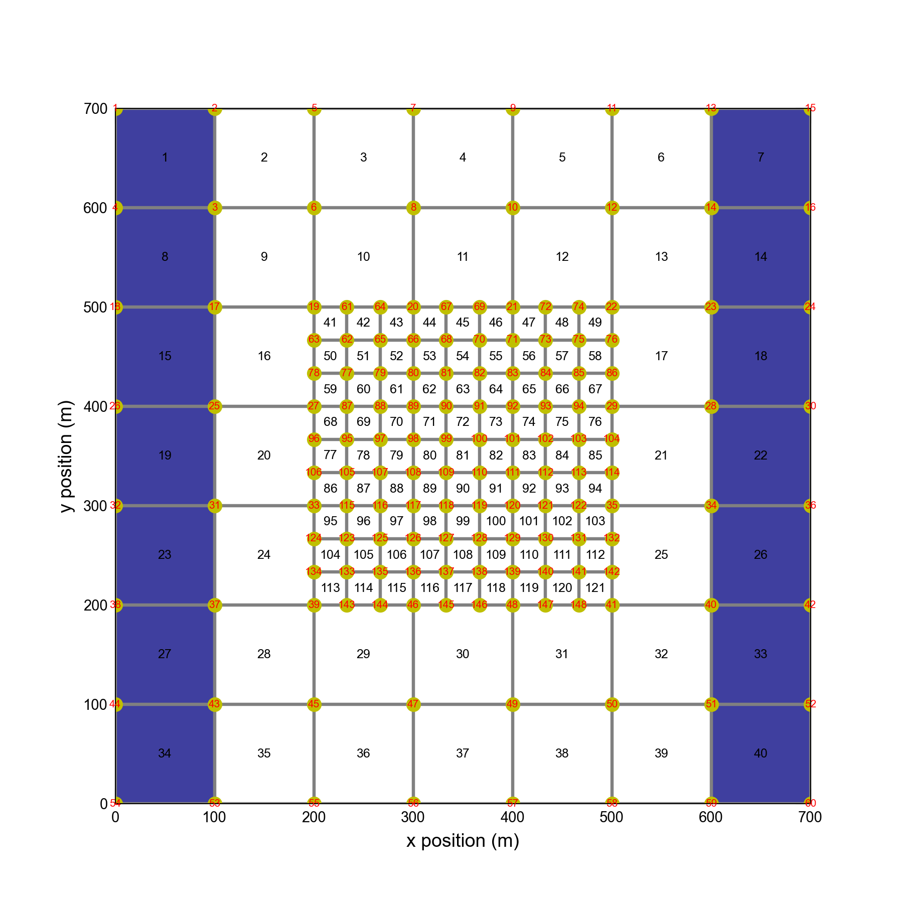
Figure 6.1 Model grid used for the nested grid problem. Constant-head cells are marked in blue. Cell numbers are shown inside each model cell. Vertices are also numbered and are shown in red.
Parameter |
Value |
|---|---|
Number of periods |
1 |
Number of layers |
1 |
Top of the model (\(m\)) |
0.0 |
Layer bottom elevations (\(m\)) |
–100.0 |
Starting head (\(m\)) |
0.0 |
Cell conversion type |
0 |
Horizontal hydraulic conductivity (\(m/d\)) |
1.0 |
6.2. Scenario Results
The nested grid problem was run with the standard groundwater flow formulation and the XT3D formulation (Provost et al., 2017) (Table 6.2).
Scenario |
Scenario Name |
Parameter |
Value |
|---|---|---|---|
1 |
ex-gwf-u1disv |
xt3d |
False |
2 |
ex-gwf-u1disv-x |
xt3d |
True |
6.2.1. Standard Groundwater Flow Formulation
Model results for the simulation with the standard groundwater flow formulation are shown in Figure 6.2. Flow is from left to right and should be perfectly one dimensional. The head surface should represent a flat plane with a value of 1.0 on the left and zero on the right. Because the configuration of a nested grid violates the control-volume finite-difference assumptions, there are errors in the simulated heads as shown in Figure 6.2B. Head errors are larger than solution tolerances.
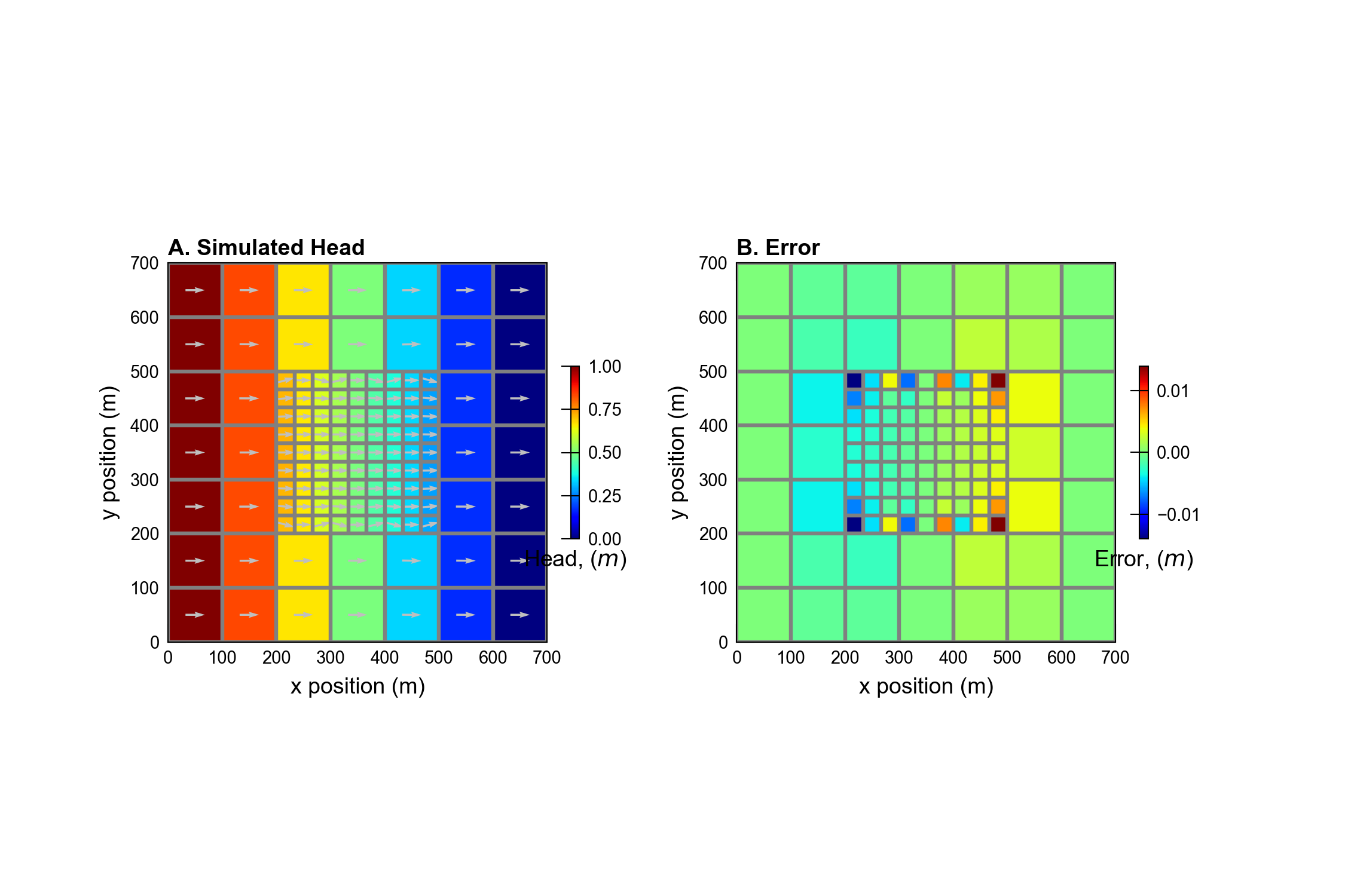
Figure 6.2 Simulated head (A) and errors in simulated head (B) for the nested grid problem simulated with the standard groundwater flow formulation.
6.2.2. XT3D
Model results for the simulation with the XT3D groundwater flow formulation (Provost et al., 2017) are shown in Figure 6.3. In this simulation, the XT3D formulation gives a much better solution than the standard groundwater flow formulation. Errors in simulated head (Figure 6.3B) are smaller than the tolerances used for the problem.
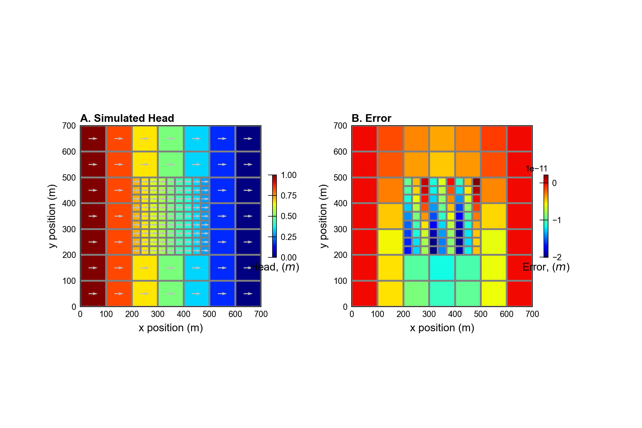
Figure 6.3 Simulated head (A) and errors in simulated head (B) for the nested grid problem simulated with the XT3D groundwater flow formulation (Provost et al., 2017).
6.3. References Cited
Panday, S., Langevin, C. D., Niswonger, R. G., Ibaraki, M., & Hughes, J. D. (2013). MODFLOW-USG version 1—an unstructured grid version of MODFLOW for simulating groundwater flow and tightly coupled processes using a control volume finite-difference formulation. Retrieved from https://pubs.usgs.gov/tm/06/a45/
Provost, A. M., Langevin, C. D., & Hughes, J. D. (2017). Documentation for the “XT3D” Option in the Node Property Flow (NPF) Package of MODFLOW 6. https://doi.org/10.3133/tm6A56
6.4. Jupyter Notebook
The Jupyter notebook used to create the MODFLOW 6 input files for this example and post-process the results is: