60. Curvilinear Groundwater Flow Model
MODFLOW 6 vertex grids specify a set of vertices that define the edges of each model cell. Two (x, y) vertex pairs are connected in the horizontal plane by a straight line to represent edges of model cells. A set of vertices can represent a curvilinear grid (Romero & Silver, 2006) by a piecewise linear representation of the curved surfaces. Curvilinear grids can represent a radial model or replicate a curved flow domain with a major change in the dominant flow path. For example, a 90\(^{\circ}\) curvilinear grid can change the dominant flow path from the x-direction to the y-direction along the same model “column.” This example demonstrates the capability of the Discretization by Vertices (DISV) Package to represent a curvilinear grid.
Using FloPy this example replicates the steady-state, curvilinear model described in (Romero & Silver, 2006) using the grid they show in Figure 3d. The original model used a modified MODFLOW-88 (McDonald & Harbaugh, 1988) code to demonstrate the ability of MODFLOW to simulate curvilinear models by distorting the model grid to use trapezoids. The results were validated against the analytical solution presented in equation 5.4 in (Crank, 1975).
60.1. Example Description
The example consists of a steady-state, 90\(^{\circ}\) curvilinear model representing a single layer, confined, homogeneous, and isotropic aquifer (Figure 60.1). The positive x-axis represents the 0\(^{\circ}\) angle and the positive y-axis is the 90\(^{\circ}\) angle. The curvilinear model is discretized by radial bands and columns. The radial bands are a piecewise linear approximation of a curve and the columns are the discretization within a radial band.
The radial band numbering starts at 1 for the inner-most band and the column number starts at 1 for the column closest to the x-axis. For MODFLOW 6, the DISV package identifies cells by the CELL2D number (\(icell2d\)). For this example, \(icell2d\) starts at radial band 1, column 1 and increases sequentially in the column direction, then the radial direction (Figure 60.1).
All vertices between two radial bands have the same radial distance from the axis origin. The inner- and outer-most vertices have a radial distance of 4 \(ft\) and 20 \(ft\), respectively. The radial distance between band vertices is 1 \(ft\) for a total of 16 curvilinear radial bands. The radial bands are discretized in 5\(^{\circ}\) increments for a total of 18 columns per band. The single model layer is 10 \(ft\) thick with a transmissivity of 0.19 \(ft^2/day\). A constant head boundary condition is assigned to the inner- and outer-most radial bands at 10 \(ft\) and 3.334 \(ft\), respectively. The remaining model properties are summarized in Table 60.1.
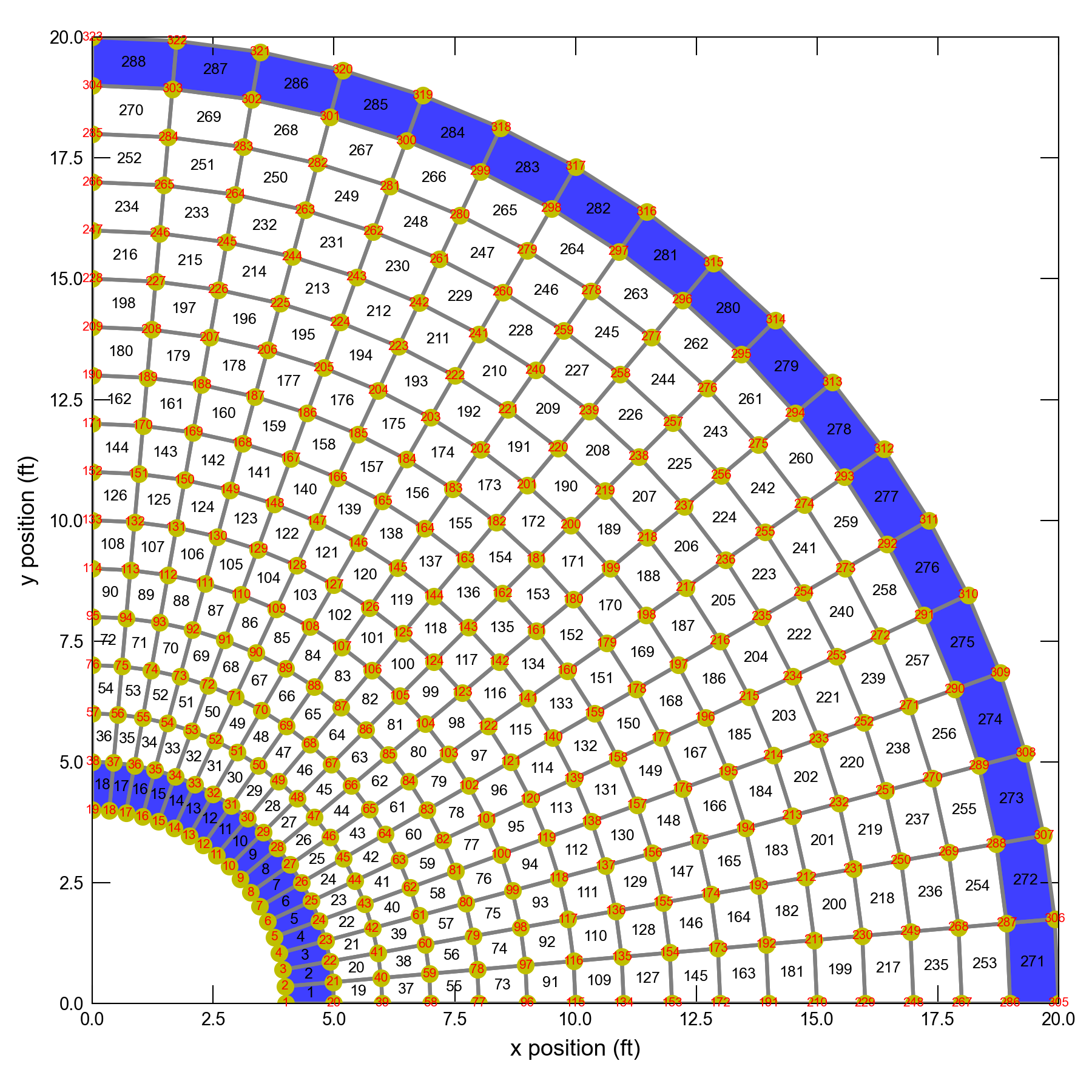
Figure 60.1 Model grid used for the 90\(^{\circ}\) curvilinear vertex model. Constant-head cells are marked in blue. The inner constant head is 10 \(ft\) and the outer constant head is 3.33 \(ft\). Cell numbers are shown inside each model cell. Vertices are also numbered and are shown in red.
Parameter |
Value |
|---|---|
Simulation Type |
Steady–State |
Number of periods |
1 |
Number of time steps |
1 |
Number of layers |
1 |
Number of radial direction cells (radial bands) |
16 |
Number of columns in radial band (ncol) |
18 |
Degree angle of column 1 boundary |
0 |
Degree angle of column ncol boundary |
90 |
Degree angle width of each column |
5 |
Model inner radius (\(ft\)) |
4 |
Model outer radius (\(ft\)) |
20 |
Model radial band width (\(ft\)) |
1 |
Top of the model (\(ft\)) |
10.0 |
Base of the model (\(ft\)) |
0.0 |
Horizontal transmissivity (\(ft^2/day\)) |
0.19 |
Horizontal hydraulic conductivity (\(ft/day\)) |
0.019 |
Inner Constant Head Boundary (\(ft\)) |
10 |
Outer Constant Head Boundary (\(ft\)) |
3.334 |
60.2. Example Results
The curvilinear vertex model is solved using one, steady state, stress period and is compared to the analytical solution (eqn. 5.4 in (Crank, 1975)). Figure 60.2 presents the MODFLOW 6 simulated head and flow lines for all model cells. Figure 60.3 presents the head solution along column 9 from all radial bands (\(icell2d\colon 9, 27, 45, \ldots, 261, 279\)) and compares it to the analytical solution. The MODFLOW 6 head solution occurs at the cell center rather than the edge, so the radial distance of the inner most head solution is 4.5 \(ft\) instead of 4 \(ft\). The MODFLOW 6 results are in agreement with the analytical solution with a relative error of 0.05% and root mean square error of 0.0037 \(ft\).
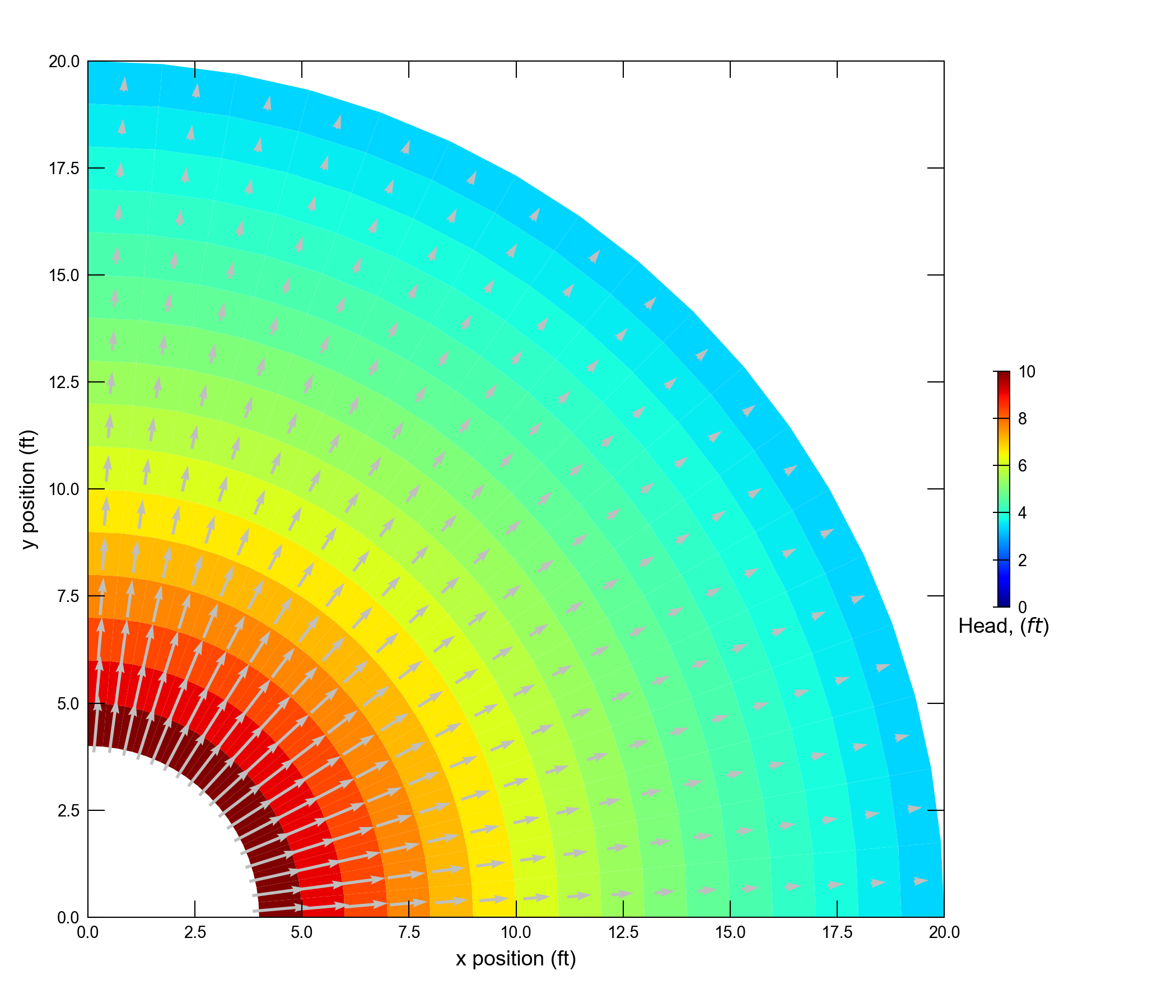
Figure 60.2 Steady state head solution and specific discharge vectors from the MODFLOW 6 curvilinear vertex model.
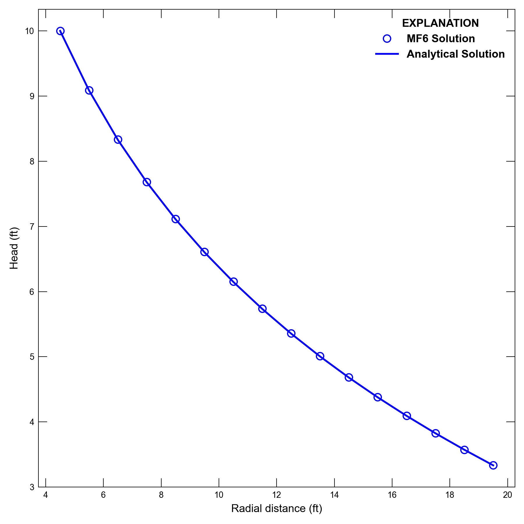
Figure 60.3 Steady state head solution from the MODFLOW 6 curvilinear vertex model (MF6) compared with the analytical solution (Crank, 1975). The MF6 head values are taken from each radial band along column 10. The radial distance of each MF6 solution is the distance from the vertex axis origin to the cell center.
60.3. References Cited
Crank, J. (1975). The mathematics of diffusion. Second edition. Oxford University Press.
McDonald, M. G., & Harbaugh, A. W. (1988). A modular three-dimensional finite-difference ground-water flow model. Retrieved from https://pubs.er.usgs.gov/publication/twri06A1
Romero, D. M., & Silver, S. E. (2006). Grid cell distortion and MODFLOW’s integrated finite-difference numerical solution. Groundwater, 44(6), 797–802. https://doi.org/10.1111/j.1745-6584.2005.00179.x
60.4. Jupyter Notebook
The Jupyter notebook used to create the MODFLOW 6 input files for this example and post-process the results is: