51. SFR1 Manual Problem 2
This problem is based on the stream-aquifer interaction problem described as test 2 by (Prudic et al., 2004). (Prudic et al., 2004) designed their test 2 problem by modifying a variant originally described by (Merritt & Konikow, 2000). The description in the text and the figures presented here are largely based on the text and figures presented by (Prudic et al., 2004). The purpose for including this problem here is to demonstrate the use of MODFLOW 6 to simulate solute transport through a coupled system consisting of an aquifer, streams, and lakes. The example requires accurate simulation of transport within the streams and lakes and also between the surface water features and the underlying aquifer.
51.1. Example description
The example problem consists of two lakes and a stream network. Figure Figure 51.1 shows the configuration of the hypothetical (but realistic) problem that was used by (Prudic et al., 2004) to demonstrate integration of the SFR1 Package with the LAK3 Package and the MODFLOW-2000 GWT Process.
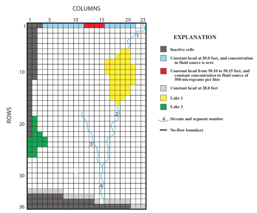
Figure 51.1 Model grid, boundary conditions and locations of lakes and streams used for the stream-lake interaction with solute transport problem. From (Prudic et al., 2004).
As described in (Prudic et al., 2004), the aquifer is moderately permeable and has homogeneous properties and uniform thickness (table Table 51.1). The aquifer was discretized into 8 layers (each 15 ft thick), 36 rows (at equal spacing of 405.7 ft), and 23 columns (at equal spacing of 403.7 ft). The flow field is represented as steady state. Uniform recharge was applied at a rate of 21 in/yr to layer 1 of the model. Two lakes are located within the model domain. Lake 1 has inflow from stream segment 1 and has outflow to stream segment 2. Lake 2 has no stream inflows or outflows. Both streams are in contact with the aquifer. Lakes are in horizontal contact with the aquifer in layer 1 around their edges and in vertical contact with the aquifer in layer 2.
Parameter |
Value |
|---|---|
Horizontal hydraulic conductivity (\(ft d^{-1}\)) |
250.0 |
Vertical hydraulic conductivity (\(ft d^{-1}\)) |
125.0 |
Storage coefficient (unitless) |
0.0 |
Aquifer thickness (\(ft\)) |
120.0 |
Porosity of mobile domain (unitless) |
0.30 |
Recharge rate (\(ft d^{-1}\)) |
4.79e-3 |
Lakebed leakance (\(ft^{-1}\)) |
1.0 |
Streambed hydraulic conductivity (\(ft d^{-1}\)) |
100.0 |
Streambed thickness (\(ft\)) |
1.0 |
Stream width (\(ft\)) |
5.0 |
Manning’s roughness coefficient (unitless) |
0.03 |
Longitudinal dispersivity (\(ft\)) |
20.0 |
Transverse horizontal dispersivity (\(ft\)) |
2.0 |
Transverse vertical dispersivity (\(ft\)) |
0.2 |
Diffusion coefficient (\(ft^2 d^{-1}\)) |
0.0 |
Initial concentration (micrograms per liter) |
0.0 |
Source concentration (micrograms per liter) |
500.0 |
Number of layers |
8 |
Number of rows |
36 |
Number of columns |
23 |
Column width (\(ft\)) |
405.665 |
Row width (\(ft\)) |
403.717 |
Layer thickness (\(ft\)) |
15.0 |
Top of the model (\(ft\)) |
100.0 |
Total simulation time (\(d\)) |
9131.0 |
The boundary conditions are illustrated in figure Figure 51.1 and were designed to produce flow that is generally from north to south. For the numerical model, constant-head conditions were specified along the northern and southern edges of the model domain, and no-flow boundaries were set along the east and west edges of the grid. In MODFLOW 6 lakes can either sit on top of the model grid, or they can be incised into the model grid as is done with previous MODFLOW versions. For this example, aquifer cells in layer 1 (Figure 51.1) that share the same space as the lake are made inactive in the model grid by setting their IDOMAIN values to zero. The constant-head boundaries were placed in all 8 layers at the map locations shown in figure Figure 51.1, with two exceptions. The first exception is related to the last downstream reach of stream segment 4. The grid cell in which the reach is located and the cell underlying it in layer 2 are both specified as active aquifer cells rather than as constant-head cells because a constant head in that cell with the stream reach would have set the gradient across the streambed. The second exception is related to the contaminant source (from treated sewage effluent), which is only introduced into the upper two model layers (that is, to a total of 8 cells). The four cells in layer 3 that underlie the contaminant source are specified as active aquifer cells rather than as constant-head cells to simulate transport beneath the source. Constant-head elevations were specified as 50.0 ft along the north boundary, except at the 4 cells in each of the upper two model layers that represent inflow from the contaminant source, where the fixed heads were 50.15 ft in the two middle cells and 50.10 ft in the two outer cells. The constant-head elevations were set to 28.0 ft along the south boundary.
The stream network consists of four segments and 38 reaches. (In MODFLOW 6 there is no concept of a segment, however the reaches are assigned names based on the segment number so that their combined flows can be compared with the results from MODFLOW-GWT.) The stream depths are calculated using Manning’s equation assuming a wide rectangular channel. For all stream reaches, the channel width was assumed constant at 5.0 ft and the roughness coefficient for the channel was 0.03. Inflows to segments 1 and 3 were specified (86,400 and 8,640 ft3/d, respectively). The inflow to stream segment 2 was equal to the outflow from lake 1, and it was calculated using Manning’s equation assuming a wide rectangular channel with a depth based on the difference between the calculated lake stage and the elevation of the top of the streambed (see (Merritt & Konikow, 2000), p. 11). The inflow to segment 4 is calculated as the sum of outflows from tributary segments 2 and 3. In MODFLOW 6 the Water Mover Package was used to route the water from the end of segment 1 into lake 1, and from the southern outlet of lake 1 into stream segment 2.
As reported by (Prudic et al., 2004) the test problem focuses on simulation of a boron plume, which results from sewage effluent. Variables related to the transport simulation are listed in table Table 51.1. For the purposes of this test, boron was assumed nonreactive. Molecular diffusion in the aquifer was assumed a negligible contributor to solute spreading at the scale of the field problem, so that hydrodynamic dispersion was related solely to mechanical dispersion, which was computed in MODFLOW 6 as a function of the specified dispersivity of the medium and the velocity of the flow field. The initial boron concentrations in the aquifer and in the lakes were assumed to be zero, and the sewage effluent concentration was assumed to be 500 micrograms/L. The source concentration in recharge was assumed to be zero and the concentration in specified inflow to stream segments 1 and 3 was also zero. The solute-transport model was run for a period of 25 years.
51.2. Example Results
The calculated steady-state head distributions in layers 1 and 2 are shown in Figure 51.2 for MODFLOW 6. This figure can be compared to figure 14 in (Prudic et al., 2004). The heads in layers 3 through 8 are almost identical to the heads shown for layer 2 (Figure 51.2). Flow is generally from north to south and predominantly horizontal. Because of recharge at the water table, however, there is a slight vertically downward flow in most areas. The lakes and streams exert a strong influence on the location and magnitude of vertical flow. In layer 2, the good hydraulic connection with the lakebed results in an almost flat horizontal hydraulic gradient in head beneath the lakes (fig. Figure 51.2). In general the simulated water table and aquifer heads simulated by MODFLOW 6 are in good agreement with those simulated by MODFLOW-2000.
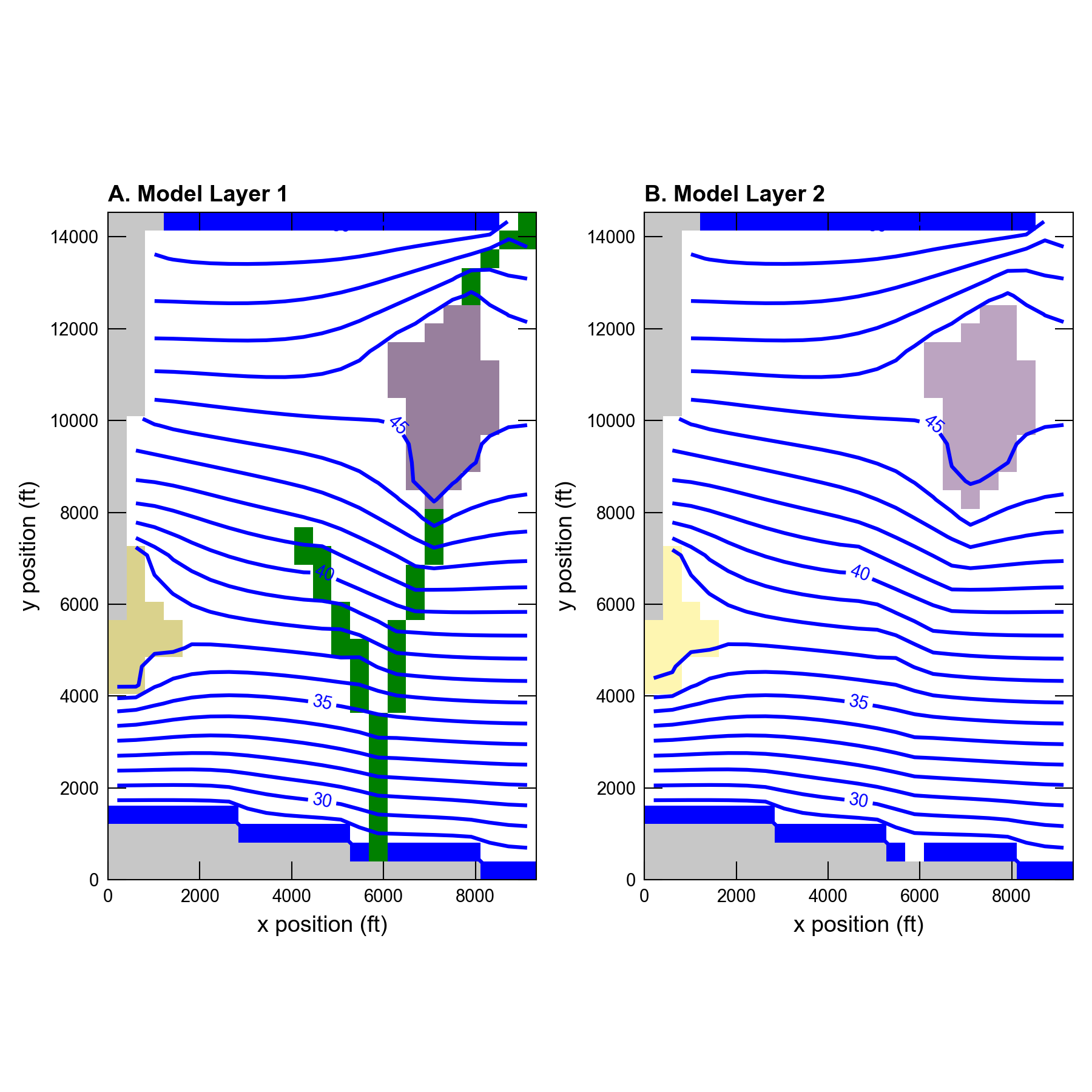
Figure 51.2 Contours of head simulated by the MODFLOW 6 GWF Model for the stream-lake interaction example. Contours are for (A) layer 1, and (B) layer 2. This figure can be compared with figure 14 in (Prudic et al., 2004), which shows head contours as simulated by MODFLOW-2000.
The MODFLOW 6 model calculated steady-state stage in lake 1 was 45.07 ft (compared to 44.97 ft in MODFLOW-GWT) and in lake 2 was 37.15 ft (compared to 37.14 ft in MODFLOW-2000). Stream segment 1 was mostly a gaining stream (leakage across streambed was from ground water), and stream segment 2 was losing such that outflow from the last reach in segment 2 was only half of the inflow from lake 1. Stream segment 3 was mostly gaining and outflow from this segment was only from groundwater leakage. Lastly, stream segment 4 was a losing stream and leakage was from the stream to the aquifer in every reach. Simulated flows between MODFLOW 6 and MODFLOW-2000 are in good qualitative agreement, however there are differences in individual flows, which can be attributed to slight differences in the way MODFLOW 6 and MODFLOW-2000 simulate lakes, streams, and groundwater flow.
For the MODFLOW 6 simulation, the 25-year period was divided into 300 time steps (compared with 1229 time steps used for the MODFLOW-GWT simulation). Advective groundwater flow was solved using the second-order implicit Total Variation Diminishing (TVD) scheme. Dispersion was solved using the XT3D approach, which was originally designed to represent full three-dimensional anisotropic groundwater flow (Provost et al., 2017). Transport through the surface water system was solved using the Lake Transport (LKT) Package, the Streamflow Transport (SFT) Package, and the Mover Transport (MVT) Package, which transfers solute between the lake and stream according to simulated flows. Additional detail on the transport parameters for the MODFLOW-GWT simulation are described in (Prudic et al., 2004) and in (Merritt & Konikow, 2000). The calculated concentration in lake 1 and in the outflow from the last reach in stream segments 2, 3, and 4 during the 25-year simulation period are shown in figure Figure 51.3 for both the MODFLOW 6 simulation and the MODFLOW-GWT simulation. Note that because stream segment 2 lost flow to ground water in all reaches and its only source was inflow from lake 1, solute concentration in the outflow from the last reach in stream segment 2 was equal to the concentration in the discharge from lake 1 (Figure 51.3). The leading edge of the plume reaches the upstream edge of lake 1 after about 4 years, at which time the concentration in the lake begins to increase rapidly. After about 22 years, the part of the plume close to the source and near the lake has stabilized and the concentration in lake 1 reaches an equilibrium concentration of 37.2 micrograms/L as simulated by MODFLOW 6 and 37.4 micrograms/L as simulated by MODFLOW-GWT. Although there are differences in the surface water concentrations simulated by MODFLOW 6 and MODFLOW-GWT, the general pattern and behavior is quite similar. Differences between the two models are generally attributed to slight differences in simulated flows as well as slight differences in how solute transport is represented. For example, MODFLOW-GWT uses the method-of-characteristics to simulate advective flow, whereas MODFLOW 6 uses an implicit TVD approach. The methods-of-characteristics approach implemented in MODFLOW-GWT is exceptional for reducing numerical dispersion, whereas the second-order TVD approach implemented in MODFLOW 6 is relatively fast and efficient, but it has more numerical dispersion than MODFLOW-GWT.
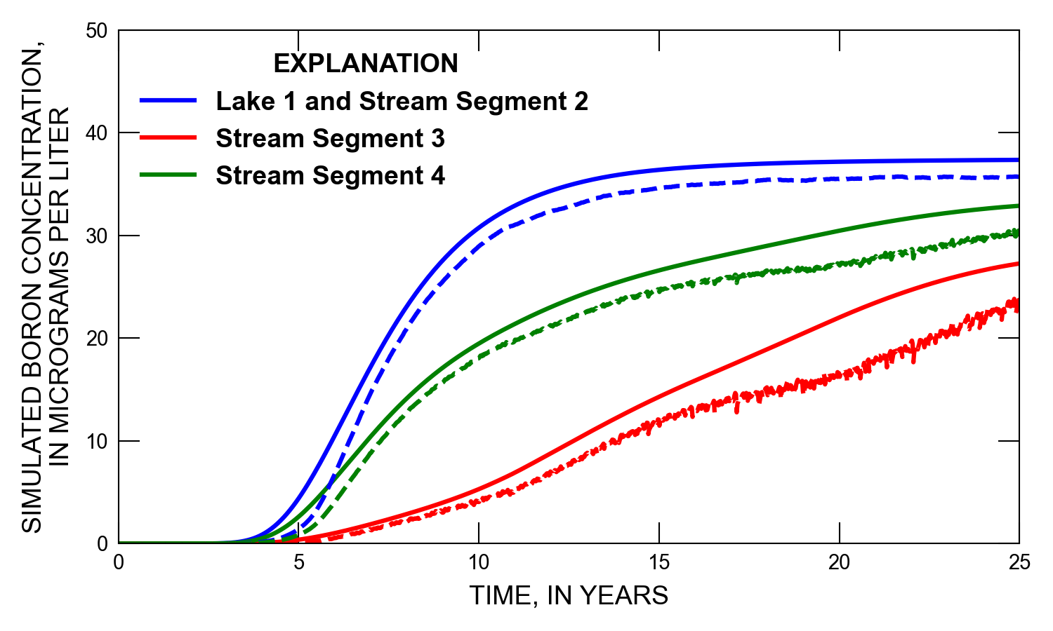
Figure 51.3 Concentration versus time simulated by MODFLOW 6 for the stream-lake interaction example. Solid lines represent the MODFLOW 6 simulated change in boron concentration in lake 1 and at the end of stream segments 2, 3, and 4. Dashed lines are results from the MODFLOW-GWT simulation (Prudic et al., 2004).
As the lake concentration increases, it in turn acts as a source of contamination to the aquifer in the areas where the lake is a source of water to the aquifer. Although the lake significantly dilutes the contaminants that enter it from the aquifer, the lake and the stream segments downstream from it in effect provide a short circuit for the relatively fast transmission of low levels of the contaminant. This is evident in Figure 51.4, which shows the computed solute distributions in layers 1, 3, 5, and 8 after 25 years. The low-concentration part of the plume emanating from the downgradient side of lake 1 has advanced farther, and is wider, than the main plume that emanated directly from the source at the north edge of the model. The influence of groundwater discharge to stream segment 3 is most apparent in the concentration pattern shown in layer 1 of figure Figure 51.4 (that is, the 25 microgram/L contour). Comparison of concentration levels at different depths in the system indicates that in the southern part of the area, concentrations generally increase with depth. In contrast, in the northern part downgradient from the source, the highest concentrations occur in layer 3. These various patterns result from the dilution effect of recharge of uncontaminated water at the water table coupled with the consequent downward component of flow, which causes the solute to move slowly downward as it migrates to the south. Solute concentrations simulated by MODFLOW 6 and shown in Figure 51.4 are generally in good agreement with those simulated by MODFLOW-GWT (figure 17 in (Prudic et al., 2004)). There are some differences, which can be attributed to the slightly different flow field and the differences in solute transport solution schemes.
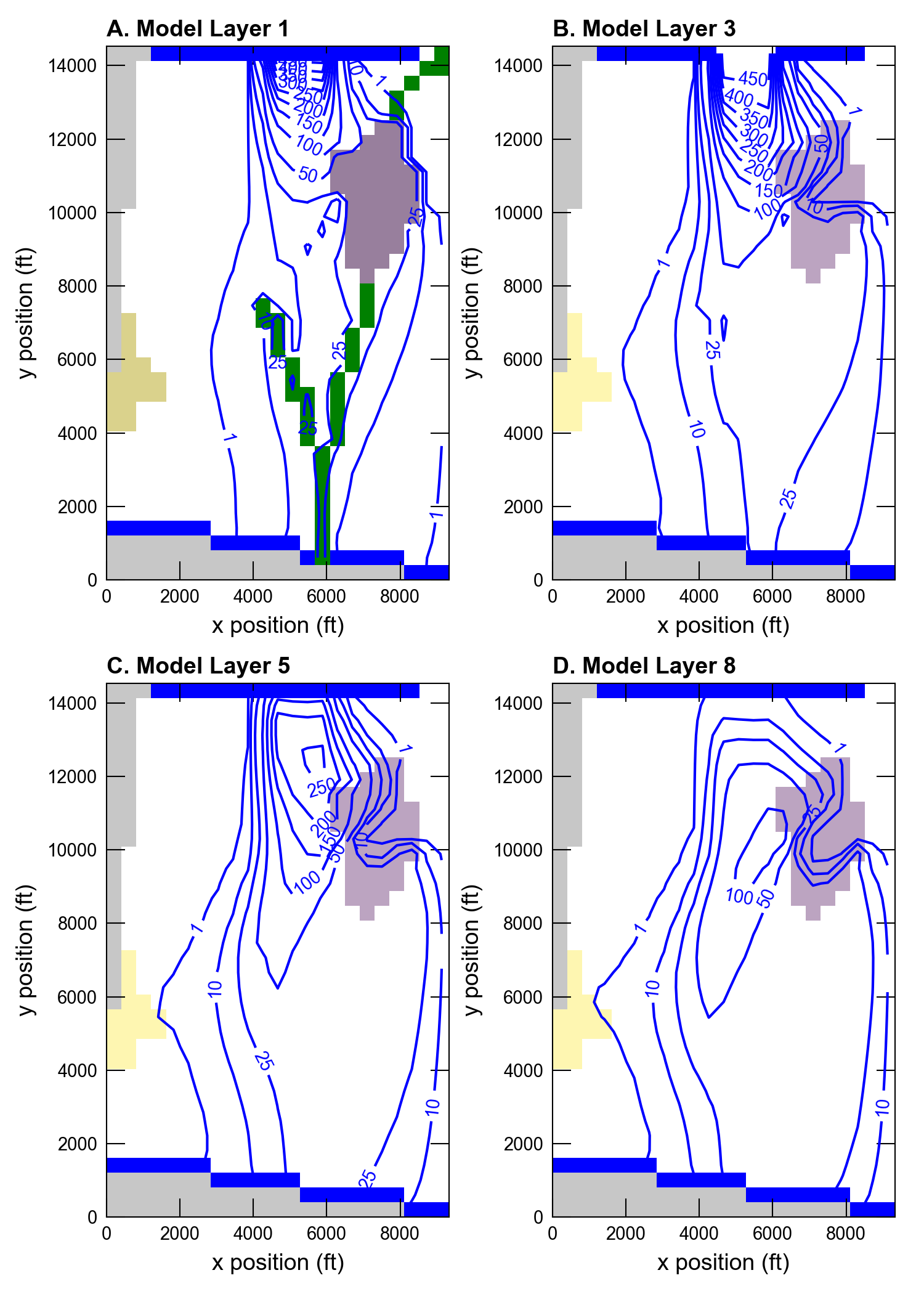
Figure 51.4 Contours of concentration simulated by the MODFLOW 6 GWT Model for the stream-lake interaction example. Contours are shown for (A) layer 1, (B) layer 3, (C) layer 5, and (D) layer 8. This figure can be compared with figure 17 in (Prudic et al., 2004), which shows an equivalent plot using model results simulated by MODFLOW-GWT.
51.3. References Cited
Merritt, M. L., & Konikow, L. F. (2000). Documentation of a computer program to simulate lake-aquifer interaction using the MODFLOW ground-water flow model and the MOC3D solute-transport model. Retrieved from https://pubs.er.usgs.gov/publication/wri004167
Provost, A. M., Langevin, C. D., & Hughes, J. D. (2017). Documentation for the “XT3D” Option in the Node Property Flow (NPF) Package of MODFLOW 6. https://doi.org/10.3133/tm6A56
Prudic, D. E., Konikow, L. F., & Banta, E. R. (2004). A new streamflow-routing (SFR1) package to simulate stream-aquifer interaction with MODFLOW-2000. Retrieved from https://pubs.er.usgs.gov/publication/ofr20041042
51.4. Jupyter Notebook
The Jupyter notebook used to create the MODFLOW 6 input files for this example and post-process the results is: