57. Stallman Problem
(Stallman, 1965) presents an analytical solution for transient heat flow in the subsurface in response to s sinusoidally varying temperature boundary imposed at land surface. The problem includes heat convection in response to downward groundwater flow. The problem also includes heat conduction through the fully saturated aquifer material. The analytical solution quantifies the temperature variation as a function of depth and time for this one-dimensional transient problem.
This section presents the results of a MODFLOW 6 simulation and the corresponding analytical solution presented by (Stallman, 1965). The MODFLOW 6 simulation includes a GWF Model and a GWT Model. Although the GWT Model was developed for solute transport, input parameters can be modified so that the GWT Model can approximate heat transport.
57.1. Example Description
The example problem presented here consists of a vertical profile from land surface (0 m) to a depth of 60 m. There are 120 model cells used to represent the profile. Groundwater flow is simulated using steady-state conditions with the top and bottom cells assigned as constant heads. The head in the top cell is given a value of 60 m and the head in the bottom cell is set to 59.701801 m. This results in a constant downward flow velocity that remains constant during the simulation.
The model simulates 10 sinusoidal periods over a total duration of 10 years (wave length = 1 year) with a total of 600 stress periods and 6 time steps per period (time step = 1 day).
For the GWT Model setup, an ambient temperature of 10 \(^o C\) is given as the initial condition. The temperature variation at the surface boundary is 5 \(^o C\) and varies with time according to \(T_{BC} = 10+5sin(2\pi t/T)\), where t is the current time and T is the wave length of one year. Solute analogs for the heat transport problem were calculated from thermal parameters. The diffusion coefficient is given as 1.02882E-06 (\(m^2/s\)), and linear sorption is activated with porosity = 0.35, bulk density = 1709.5 (\(kg/m^3\)) and the distribution coefficient = 0.000191663. Model parameters used for this example are shown in Table 57.1.
Parameter |
Value |
|---|---|
Number of periods |
600 |
Number of time steps |
6 |
Simulation time length (\(s\)) |
525600 |
Number of layers |
120 |
Number of rows |
1 |
Number of columns |
1 |
Length of system (\(m\)) |
60.0 |
Column width (\(m\)) |
1.0 |
Row width (\(m\)) |
1.0 |
Layer thickness |
ranges from 0.1 to 1 |
Top of the model (\(m\)) |
60.0 |
Hydraulic conductivity (\(m s^{-1}\)) |
1.0e-4 |
Porosity (unitless) |
0.35 |
Longitudinal dispersivity (\(m\)) |
0.0 |
Transverse dispersivity (\(m\)) |
0.0 |
Diffusion coefficient (\(m s^{-1}\)) |
1.02882e-06 |
Ambient temperature (\(^o C\)) |
10 |
Temperature variation (\(^o C\)) |
5 |
Bulk density (\(kg/m^3\)) |
2630 |
Distribution coefficient (unitless) |
0.000191663 |
57.2. Example Results
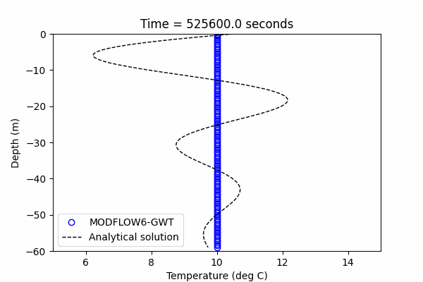
The simulated temperature profile from MODFLOW 6 shows good agreement with the temperature profile from the Stallman analytical solution for a simulation time of 9.02 yr (Figure 57.1).
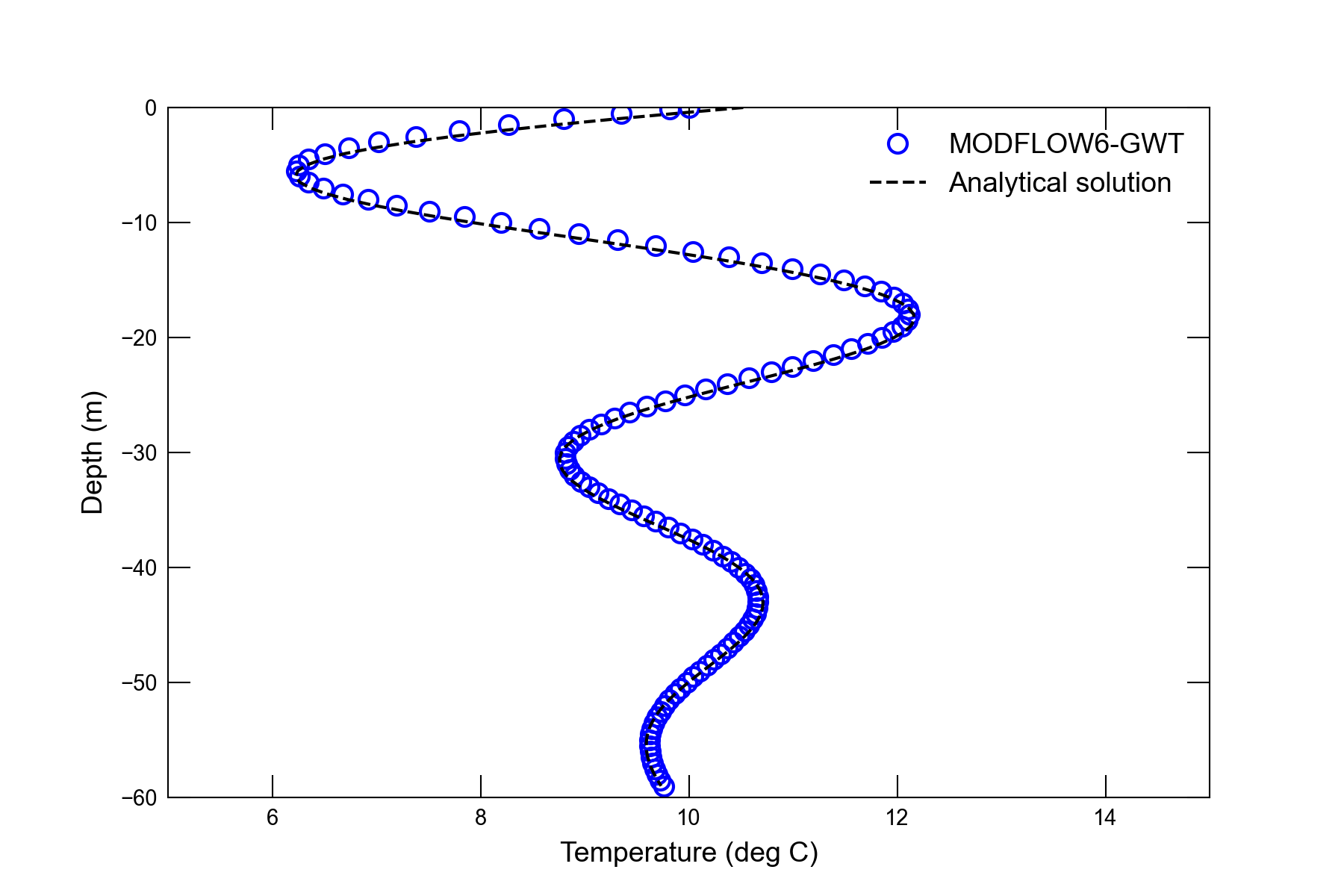
Figure 57.1 Comparison of the temperature profile simulated with MODFLOW 6(blue circles) and calculated with the (Stallman, 1965) analytical solution (dashed line).
57.3. References Cited
Stallman, R. (1965). Steady one-dimensional fluid flow in a semi-infinite porous medium with sinusoidal surface temperature. Journal of Geophysical Research, 70(12), 2821–2827. https://doi.org/10.1029/JZ070i012p02821
57.4. Animation
Animation of model results: