23. LGR with MVR and SFR
This example is based on LGR2 Problem 3 in (Mehl & Hill, 2013), which includes two models arranged in a nested parent-child grid setup, where the parent model uses a coarse grid that surrounds the finely-gridded child model (Figure 23.1). Parent-child model setups limit grid refinement to localized regions of interest within large model domains to keep model runtimes to a minimum. Owing to the relative ease of setup for this type of model arrangement in MODFLOW 6, particularly when developing a model (i.e., simulation) with a support utility like flopy (Bakker et al., 2016), the use of multi-model arrangements necessitates a generalized supporting package like MVR to transfer water among features within a simulation. To demonstrate, this example uses MVR to cascade streamflow from an upstream SFR reach in the parent model to a downstream SFR reach in the child model. Further downstream MVR again cascades streamflow from the last child model SFR reach to the appropriate SFR reach in the parent model.
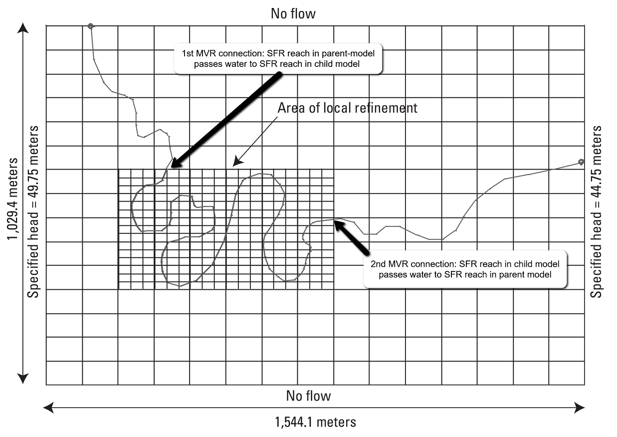
Figure 23.1 Plan view of a three-dimensional aquifer system used to test the local grid refinement method in MODFLOW 6. A 15\(\times\)15 horizontal grid discretization is shown for the parent grid and the locally refined grid (15\(\times\)18) spacing is equivalent to a 45\(\times\)45 discretization over the whole domain. Two between-model MVR connections are invoked for the SFR packages (parent and child) where the river crosses between domains
23.1. Example description
The parent model is 15 rows by 15 columns by 3 layers with the child model occupying a 5 row by 6 column by 2 layer portion of the parent grid as shown in Figure 23.1. The child model applies a 3:1 refinement to each parent grid cell, including in the vertical direction, resulting in a 15 row by 18 column by 6 layer child model. In this way, each parent grid cell is replaced by 27 (\(3^3\)) child model grid cells. Aquifer properties are uniform and equal throughout both model domains. Interested readers are referred to (Mehl & Hill, 2013) for additional model details.
Parameter |
Value |
|---|---|
Number of layers in parent model |
3 |
Number of rows in parent model |
15 |
Number of columns in parent model |
15 |
Parent model column width (\(m\)) |
102.94 |
Parent model row width (\(m\)) |
68.63 |
Number of child model columns per parent model columns |
5 |
Number of child model rows per parent model rows |
5 |
Child model column width (\(m\)) |
20.588 |
Child model row width (\(m\)) |
13.725 |
Horizontal hydraulic conductivity (\(m/d\)) |
1.0 |
Vertical hydraulic conductivity (\(m/d\)) |
1.0 |
Figure 23.2 demonstrates that both MVR connections transfer streamflow to the appropriate stream reach in the receiving downstream model. This is evidenced by the continuous and smooth downward trend in streamflow at the first MVR connection as well as by the uninterrupted upward trend in streamflow at the second MVR connection.
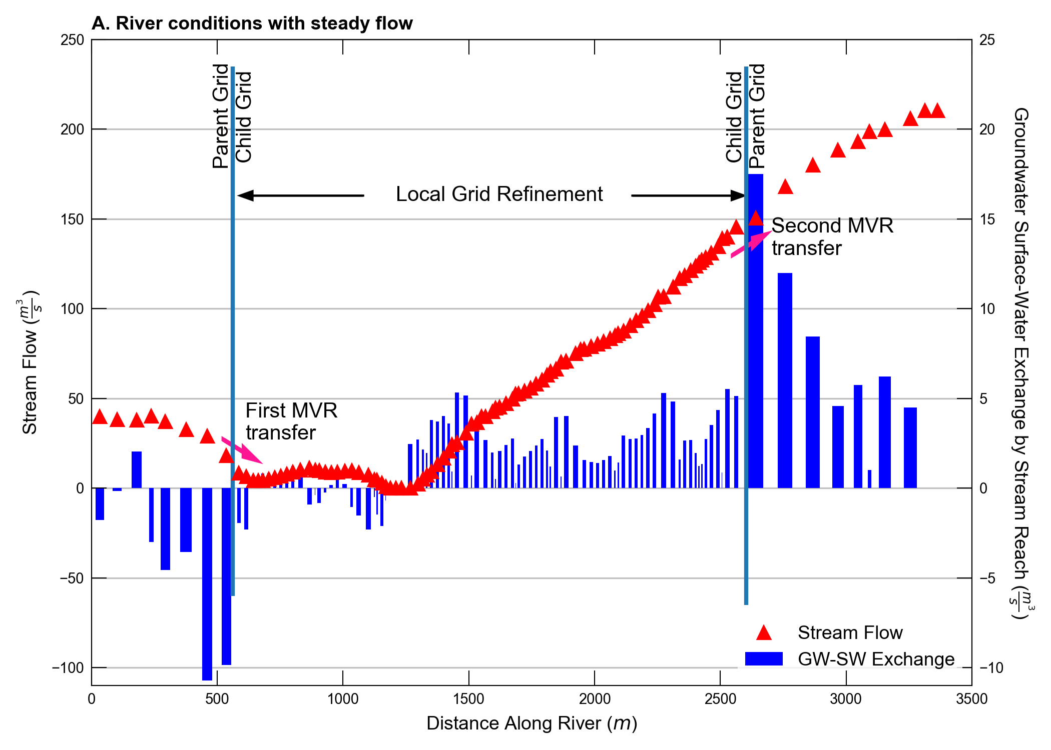
Figure 23.2 Simulated streamflow and groundwater surface-water exchange for each stream reach in Figure 23.1. The transfer of water between adjacent stream reaches in the parent versus child models occurs at locations identified by the vertical black lines on the plot. Bar widths are indicative of the relative stream reach lengths within the host grid cell (figure Figure 23.1).
23.2. References Cited
Bakker, M., Post, V., Langevin, C. D., Hughes, J. D., White, J. T., Starn, J. J., & Fienen, M. N. (2016). Scripting MODFLOW model development using Python and FloPy. Groundwater, 54(5), 733–739. https://doi.org/10.1111/gwat.12413
Mehl, S. W., & Hill, M. C. (2013). MODFLOW–LGR Documentation of Ghost Node Local Grid Refinement (LGR2) for Multiple Areas and the Boundary Flow and Head (BFH2) Package. https://doi.org/10.3133/tm6A44
23.3. Jupyter Notebook
The Jupyter notebook used to create the MODFLOW 6 input files for this example and post-process the results is: