54. Salt Lake Problem
The salt lake problem was suggested by (Simmons et al., 1999) as a comprehensive benchmark test for variable-density groundwater flow models. The problem is based on dense salt fingers that descend from an evaporating salt lake. Although an analytical solution is not available for the salt lake problem, an equivalent Hele-Shaw analysis was performed in the laboratory to investigate the movement of dense salt fingers (Wooding, Tyler, & White, 1997; Wooding, Tyler, White, & Anderson, 1997). In addition to the SUTRA simulation, this salt lake problem was simulated by (Langevin et al., 2003) using the MODFLOW-based SEAWAT-2000 program. The approach described by (Langevin et al., 2003) is followed here to reproduce the salt lake problem with MODFLOW 6.
54.1. Example description
Model parameters used for the MODFLOW 6 simulation of the salt lake problem are shown in Table 54.1 The model grid and boundary conditions used for the MODFLOW 6 simulation are shown in Figure 54.1. The model grid consists of 135 columns and 57 layers. To accurately capture the number and growth of salt fingers, the model grid has an increased level of resolution beneath the evaporative boundary. The evaporative boundary is represented in the model by using the Recharge (RCH) Package and specifying a negative recharge rate. (Simmons et al., 1999) describe the method for applying the SUTRA code to the salt lake problem. A random numerical perturbation was required to match the formation of the salt fingers observed in the Hele-Shaw experiment. Concentrations along the evaporative boundary were randomly assigned for each node and for each time step. A similar approach is used here for the MODFLOW 6 simulation, except that the random variations are not reassigned each time step. The inflow boundary is represented using constant-head cells with a constant inflow concentration. The MODFLOW 6 model was run for 24,000 seconds (400 minutes) using 60-second transport timesteps.
Parameter |
Value |
|---|---|
Number of periods |
1 |
Number of time steps |
400 |
Simulation time length (\(s\)) |
24000 |
Number of layers |
57 |
Number of rows |
1 |
Number of columns |
135 |
Length of system (\(mm\)) |
150.0 |
Column width (\(mm\)) |
ranges from 0.75 to 1.5 |
Row width (\(mm\)) |
1.5 |
Layer thickness |
ranges from 0.75 to 1.5 |
Top of the model (\(mm\)) |
75.0 |
Hydraulic conductivity (\(mm s^{-1}\)) |
3.05 |
Specific storage (\(mm^{-1}\)) |
3.8e-10 |
Reference density |
0.001065 |
Density and concentration slope |
0.646 |
Initial and inflow concentration (\(g L^{-1}\)) |
8.4e-5 |
Saturated concentration (\(g L^{-1}\)) |
1.1e-4 |
Porosity (unitless) |
1.0 |
Evaporation rate (\(mm s^{-1}\)) |
1.03e-3 |
Longitudinal dispersivity (\(mm\)) |
9.0e-7 |
Transverse dispersivity (\(mm\)) |
9.0e-7 |
Diffusion coefficient (\(mm s^{-1}\)) |
9.0e-4 |
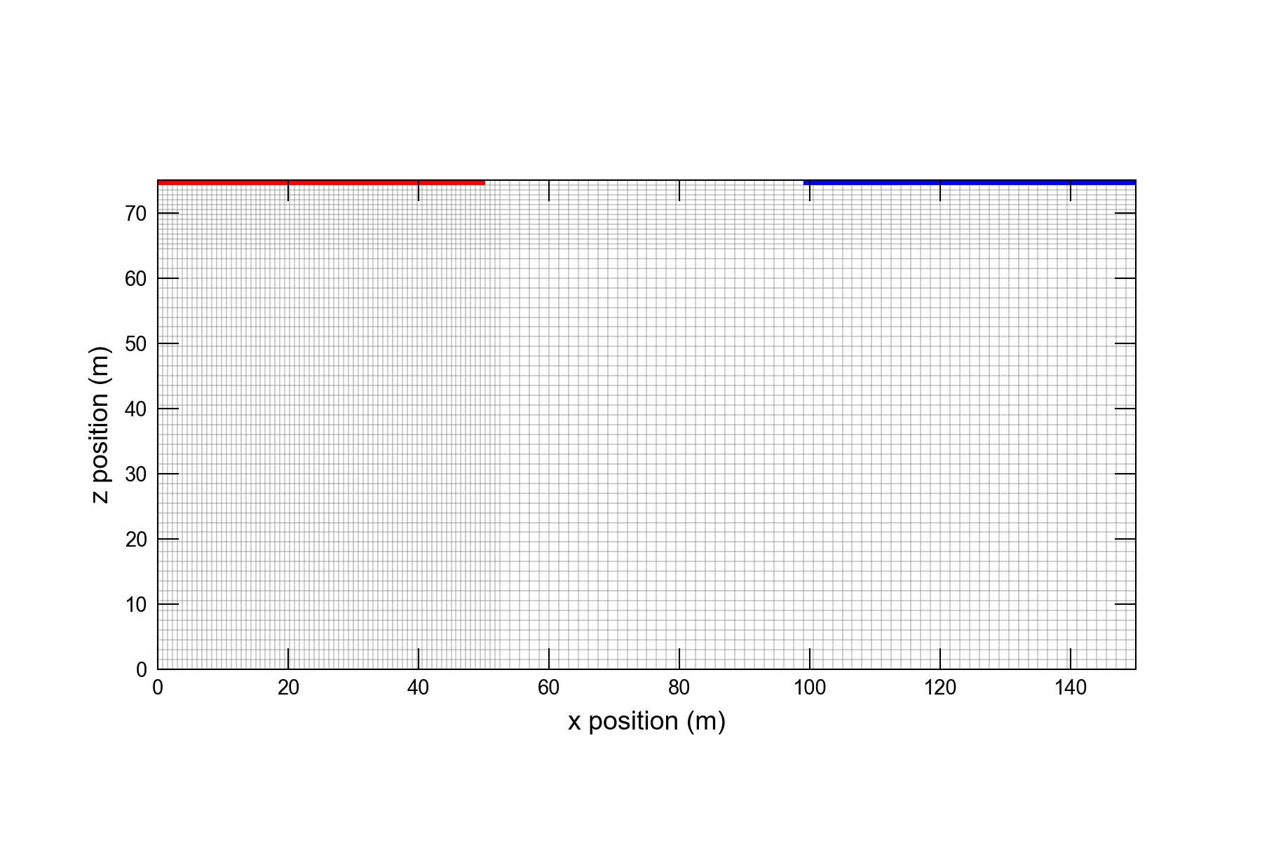
Figure 54.1 Model grid and boundary conditions used for the salt lake problem. Evaporation occurs from the cells highlighted in red. Inflow into the model grid occurs through the constant-head cells shown in blue.
54.2. Example Results
The salt lake problem represents a complex system of salt fingers that form, descend, and then coalesce due to the larger-scale flow system. Although the results from MODFLOW 6 are not identical with the results from the Hele-Shaw experiment, MODFLOW 6 seems capable of representing the growth rate and number of salt fingers (Figure 54.2). In the experiment and model, six or seven salt fingers are initially produced, of which only two persist. The rate of descent is similar for both the experiment and model.
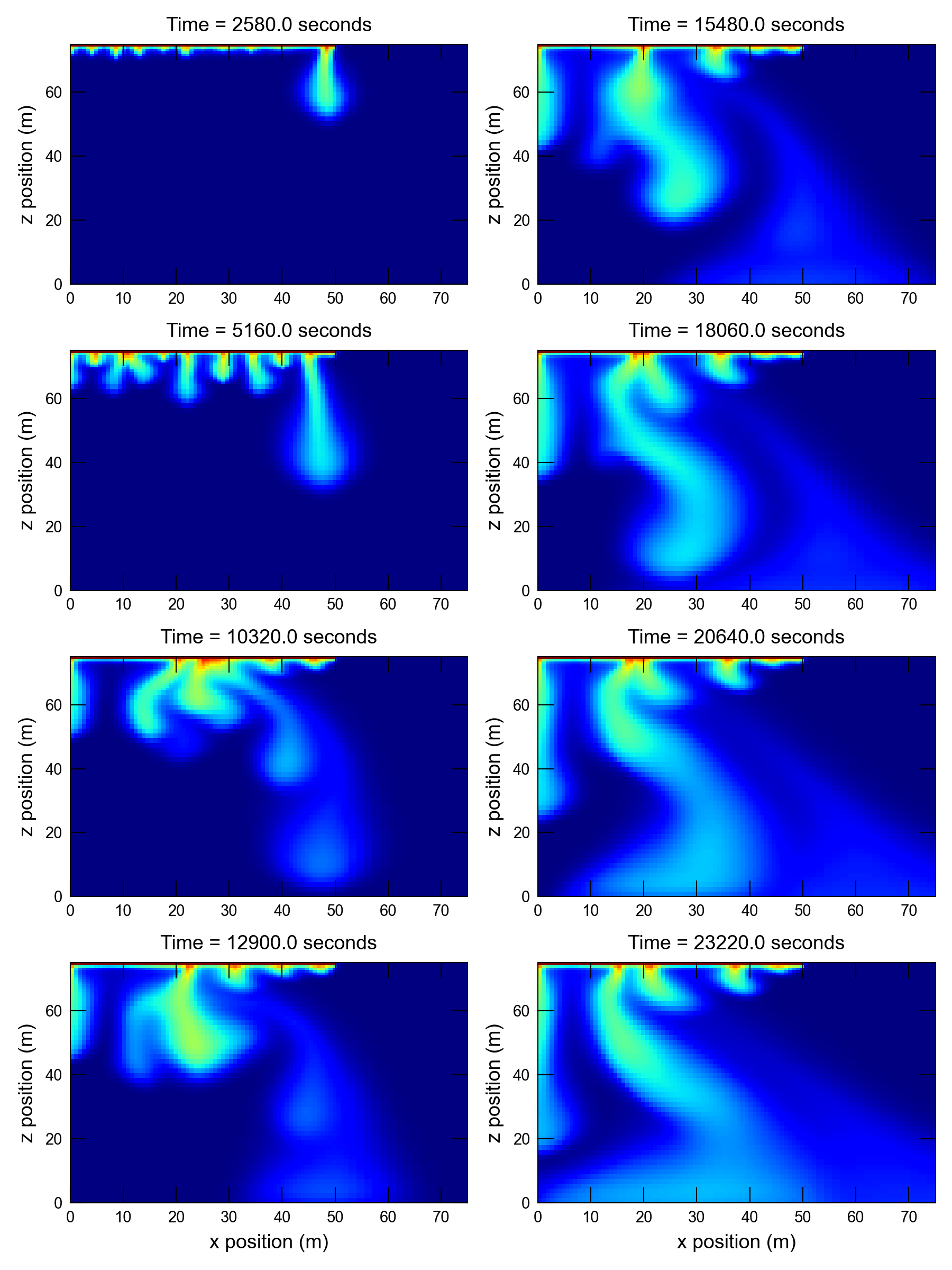
Figure 54.2 Color-shaded plots of concentration simulated by MODFLOW 6 for the (Simmons et al., 1999) problem involving density-driven groundwater flow and solute transport. Panels can be compared with the panels shown for the Hele-Shaw experient (Wooding, Tyler, White, & Anderson, 1997) and for the SEAWAT-2000 numerical simulation (Langevin et al., 2003).
54.3. References Cited
Langevin, C. D., Shoemaker, W. B., & Guo, W. (2003). MODFLOW-2000 the u.s. Geological survey modular ground-water model–documentation of the SEAWAT-2000 version with the Variable-Density Flow Process (VDF) and the Integrated MT3DMS Transport Process (IMT). U.S. Geological Survey. Retrieved from https://pubs.er.usgs.gov/publication/ofr03426
Simmons, C. T., Narayan, K. A., & Wooding, R. A. (1999). On a test case for density-dependent groundwater flow and solute transport models: The Salt Lake Problem. Water Resources Research, 35(12), 3607–3620. https://doi.org/10.1029/1999WR900254
Wooding, R. A., Tyler, S. W., & White, I. (1997). Convection in groundwater below an evaporating Salt Lake–1. Onset of instability. Water Resources Research, 33(6), 1199–1217. https://doi.org/10.1029/96WR03533
Wooding, R. A., Tyler, S. W., White, I., & Anderson, P. A. (1997). Convection in groundwater below an evaporating Salt Lake–2. Evolution of fingers or plumes. Water Resources Research, 33(6), 1219–1228. https://doi.org/10.1029/96WR03534
54.4. Animation
Animation of model results: