1. TWRI
This example is a modified version of the original MODFLOW example (TWRI) described in (McDonald & Harbaugh, 1988) and duplicated in (Harbaugh & McDonald, 1996). This problem is also is distributed with MODFLOW-2005 (Harbaugh, 2005). The problem has been modified from a quasi-3D problem, where confining beds are not explicitly simulated, to an equivalent three-dimensional problem.
1.1. Example Description
There are three simulated aquifers, which are separated from each other by confining layers (Figure 1.1). The confining beds are 50 \(ft\) thick and are explicitly simulated as model layers 2 and 4, respectively. Each layer is a square 75,000 \(ft\) on a side and is divided into a grid with 15 rows and 15 columns, which forms squares 5,000 \(ft\) on a side. A single steady-stress period with a total length of 86,400 seconds (1 day) is simulated.
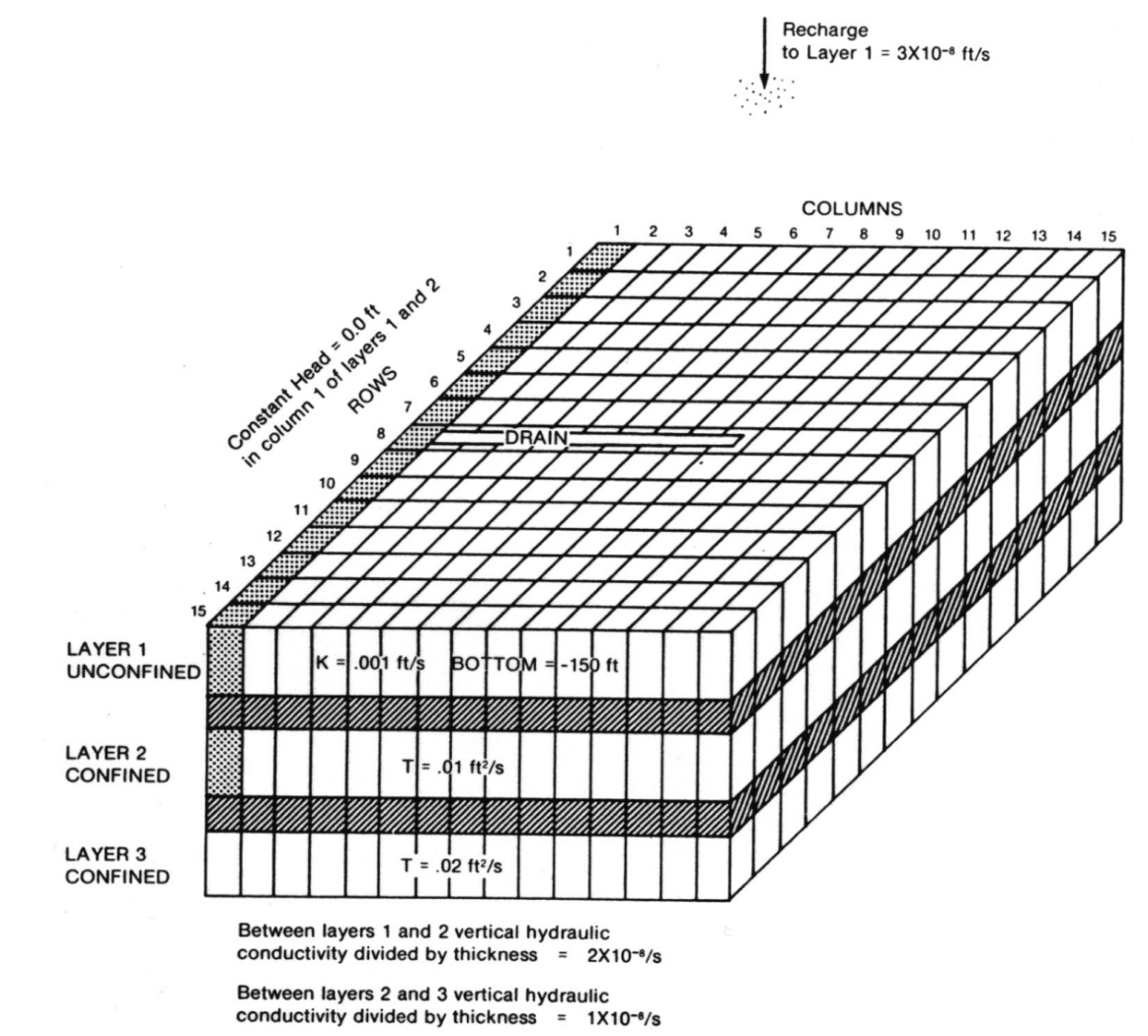
Figure 1.1 Illustration of the system simulated in the TWRI example problem, from (McDonald & Harbaugh, 1988).
The transmissivity of the middle and lower aquifers (Figure 1.1) was converted to a horizontal hydraulic conductivity using the layer thickness (Table 1.1). The vertical hydraulic conductivity in the aquifers was set equal to the horizontal hydraulic conductivity. The vertical hydraulic conductivity of the confining units was calculated from the vertical conductance of the confining beds defined in the original problem and the confining unit thickness (Table 1.1); the horizontal hydraulic conductivity of the confining bed was set to the vertical hydraulic conductivity and results in vertical flow in the confining unit.
Parameter |
Value |
|---|---|
Number of periods |
1 |
Number of layers |
5 |
Number of columns |
15 |
Number of rows |
15 |
Column width (\(ft\)) |
5000.0 |
Row width (\(ft\)) |
5000.0 |
Top of the model (\(ft\)) |
200.0 |
Layer bottom elevations (\(ft\)) |
–150.0, –200.0, –300.0, –350.0, –450.0 |
Starting head (\(ft\)) |
0.0 |
Cell conversion type |
1, 0, 0, 0, 0 |
Horizontal hydraulic conductivity (\(ft/s\)) |
1.0e-3, 1.0e-8, 1.0e-4, 5.0e-7, 2.0e-4 |
Vertical hydraulic conductivity (\(ft/s\)) |
1.0e-3, 1.0e-8, 1.0e-4, 5.0e-7, 2.0e-4 |
Recharge rate (\(ft/s\)) |
3e-8 |
An initial head of zero \(ft\) was specified in all model layers. Any initial head exceeding the bottom of model layer 1 (-150 \(ft\)) could be specified since the model is steady-state.
Flow into the system is from infiltration from precipitation and was represented using the recharge (RCH) package. A constant recharge rate of \(3 \times 10^{-7}\) \(ft/s\) was specified for every cell in model layer 1. Flow out of the model is from buried drain tubes represented by drain (DRN) package cells in model layer 1, discharging wells represented by well (WEL) package cells in all three aquifers, and a lake represented by constant head (CHD) packages cells in the unconfined and middle aquifers (Figure 1.1).
1.2. Example Results
Simulated results in the unconfined, middle, and lower aquifers are shown in Figure 1.2. Simulated results for a quasi-3D MODFLOW-2005 simulation are also shown in Figure 1.2. MODFLOW 6 and MODFLOW-2005 results differ by less that 0.05 \(ft\) in any aquifer unit.
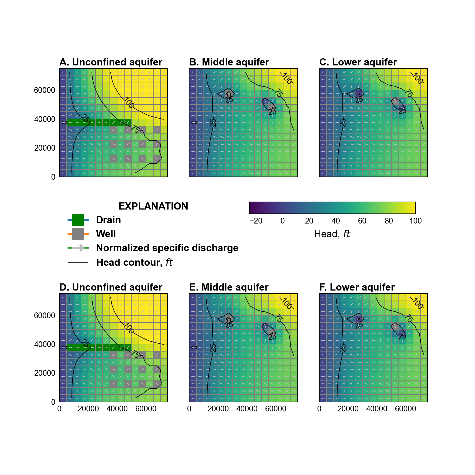
Figure 1.2 Simulated water levels and normalized specific discharge vectors in the unconfined, upper, and lower aquifers. A. MODFLOW 6 unconfined aquifer results. B. MODFLOW 6 middle aquifer results. C. MODFLOW 6 lower aquifer results. D. MODFLOW-2005 unconfined aquifer results. E. MODFLOW-2005 middle aquifer results. F. MODFLOW-2005 lower aquifer results.
1.3. References Cited
Harbaugh, A. W. (2005). MODFLOW-2005, the U.S. Geological Survey modular ground-water model—the Ground-Water Flow Process. Retrieved from https://pubs.usgs.gov/tm/2005/tm6A16/
Harbaugh, A. W., & McDonald, M. G. (1996). User’s documentation for MODFLOW-96, an update to the U.S. Geological Survey modular finite-difference ground-water flow model.
McDonald, M. G., & Harbaugh, A. W. (1988). A modular three-dimensional finite-difference ground-water flow model. Retrieved from https://pubs.er.usgs.gov/publication/twri06A1
1.4. Jupyter Notebook
The Jupyter notebook used to create the MODFLOW 6 input files for this example and post-process the results is: