5. Flow and Head Boundary (FHB) Package Replication
This example shows how the time series capability in MODFLOW 6 can be combined with the constant-head (CHD) and Well (WEL) Packages to replicate the capabilities of the Flow and Head Boundary (FHB) Package in previous versions of MODFLOW. This synthetic example problem has been released with previous MODFLOW versions, such as MODFLOW-2005 (Harbaugh, 2005) and was first described by (Leake & Lilly, 1997).
5.1. Example Description
The problem consists of a very simple single-layer model representing a confined aquifer. The grid consists of 3 rows and 10 columns. Each cell is 1000 \(m\) on a side. There are three transient stress periods with lengths of 400, 200, and 400 days. There are 10, 4, and 6 time steps per stress period. Model parameters are listed in Table 5.1.
Parameter |
Value |
|---|---|
Number of periods |
3 |
Number of layers |
1 |
Number of columns |
10 |
Number of rows |
3 |
Column width (\(m\)) |
1000.0 |
Row width (\(m\)) |
1000.0 |
Top of the model (\(m\)) |
50.0 |
Layer bottom elevations (\(m\)) |
–200.0 |
Starting head (\(m\)) |
0.0 |
Cell conversion type |
0 |
Horizontal hydraulic conductivity (\(m/d\)) |
20.0 |
Specific storage (\(/m\)) |
0.01 |
An initial head of 0 \(m\) was specified for the model. The value is important as the model begins with a transient stress period.
The model demonstrates use of the CHD and WEL packages. Locations for these boundaries are shown in Figure 5.1. Both of these packages use time varying values for the constant head and the well flow rate.
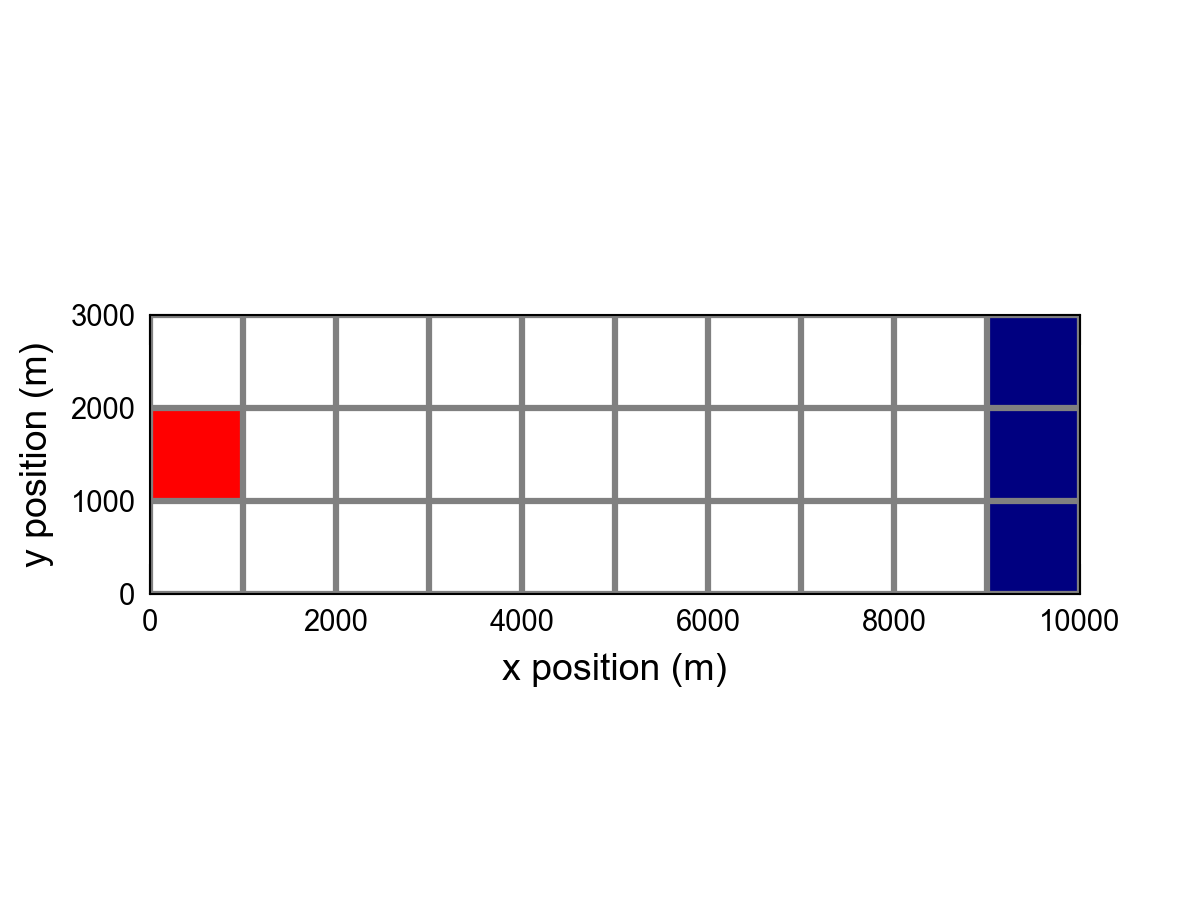
Figure 5.1 Model grid and boundary conditions used for the FHB example problem.
5.2. Example Results
The observation capability in MODFLOW 6 was used to extract time series of simulated heads and flows. Time series of model results are shown in Figure 5.2 and Figure 5.3.
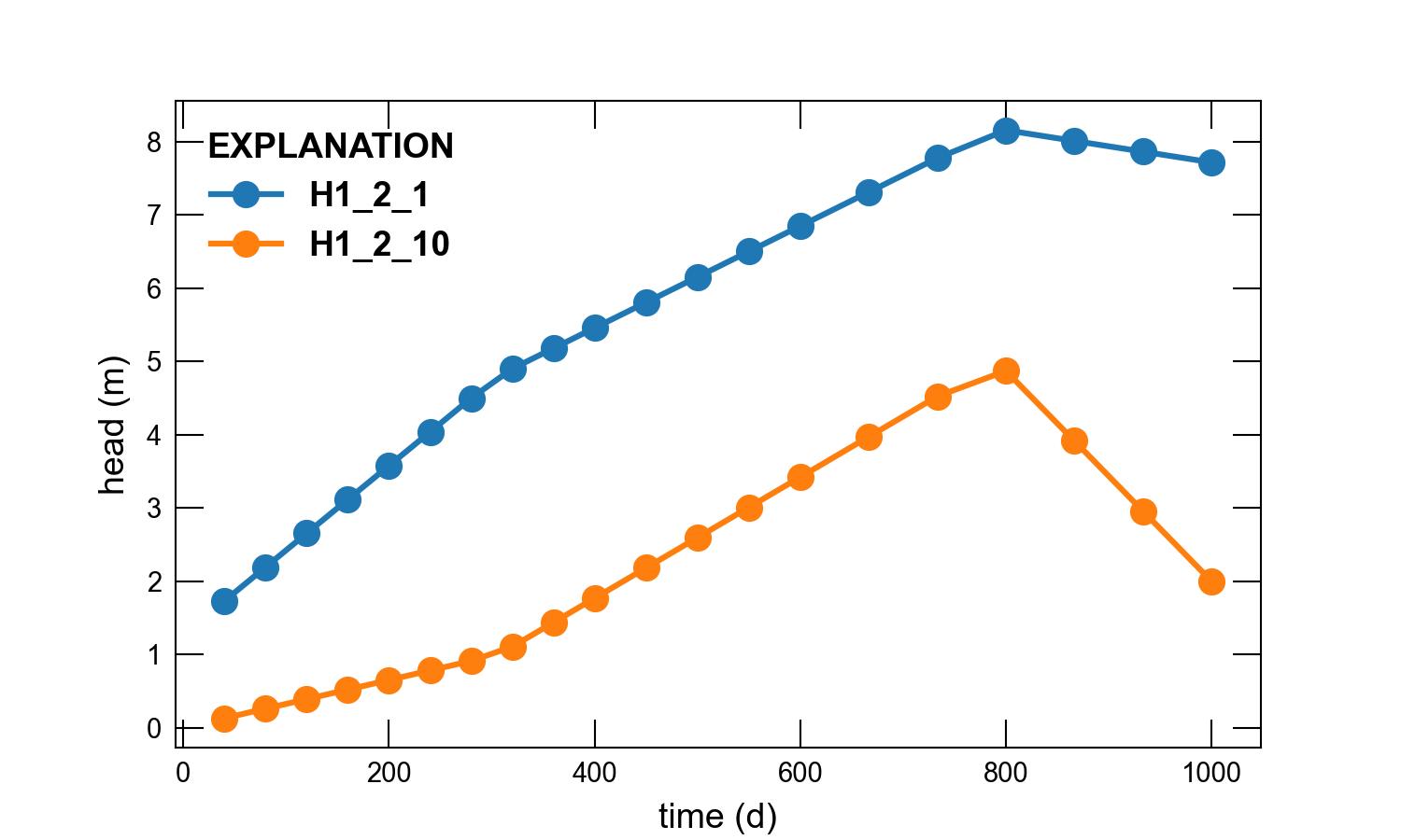
Figure 5.2 Simulated groundwater head in model cells (1, 2, 1) and (1, 2, 10).
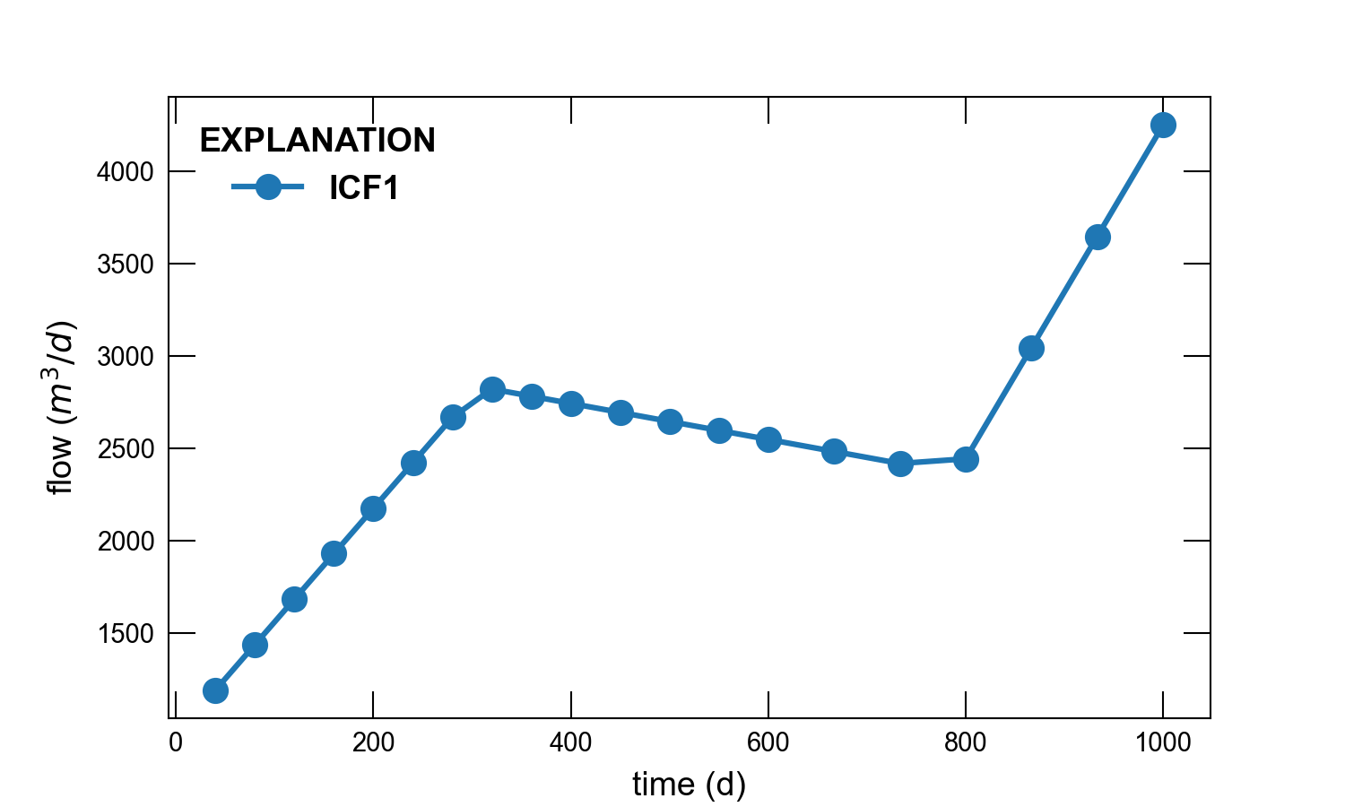
Figure 5.3 Simulated groundwater flow for model cell (1, 2, 2) and its connection with model cell (1, 2, 1). Positive values indicate flow into model cell (1, 2, 2).
5.3. References Cited
Harbaugh, A. W. (2005). MODFLOW-2005, the U.S. Geological Survey modular ground-water model—the Ground-Water Flow Process. Retrieved from https://pubs.usgs.gov/tm/2005/tm6A16/
Leake, S. A., & Lilly, M. R. (1997). Documentation of computer program (FHB1) for assignment of transient specified-flow and specified-head boundaries in applications of the modular finite-diference ground-water flow model (MODFLOW). Retrieved from https://pubs.er.usgs.gov/publication/ofr97571
5.4. Jupyter Notebook
The Jupyter notebook used to create the MODFLOW 6 input files for this example and post-process the results is: