26. Elastic Aquifer Loading
This problem simulates elastic compaction of aquifer materials in response to the loading of an aquifer by a passing train. Water-level responses were simulated for an eastbound train leaving the Smithtown Station in Long Island, New York at 13:04 on April 23, 1937 (Jacob, 1939).
26.1. Example Description
The problem is simulated as a two-dimensional half-cell cross-section model. The model grid for this problem consists of three layers, 1 row, and 35 columns (Figure 26.1). The model layers were defined based on hydrostratigraphic information in (Jacob, 1939). The upper and lower layer represent an unconfined upper aquifer and confined lower aquifer separated by a confining unit (Figure 26.1B). The upper and lower aquifers are composed of sand and gravel, respectively, and the confining unit is composed of clay.
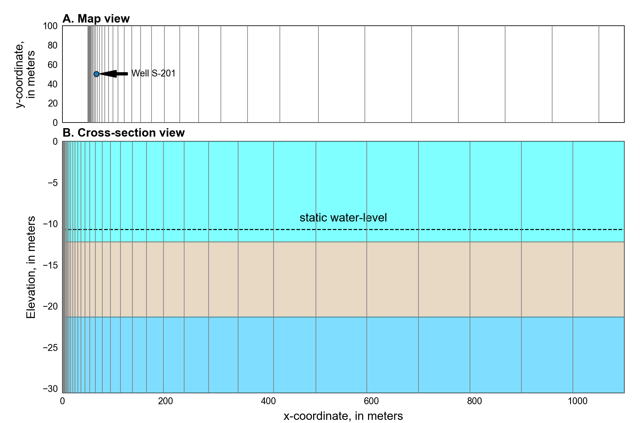
Figure 26.1 Diagram showing the model domain for the elastic aquifer loading problem. A, plan view, and B, cross-section view
The model has a top elevation of 0 meters and layer bottom elevations of -12.2, -21.3, and -30.5 meters, for layers 1, 2, and 3 respectively. DELR increases from 0.5 to 98.9 meters in columns 1 to 30, using a multiplier of 1.2; a DELR value of 100 meters is specified in columns 31 to 35. DELC is specified with a constant value of 100.6 meters and is based on the an estimate of the total length of the train (Table 26.1). The simulation consists of two stress periods. The first stress period is steady-state with a single time step and is 0.5 seconds in length. The second stress period is transient, 58.5 seconds in length, and is divided into 117 equally sized time steps.
Type |
Number |
Length, in meters |
Weight, in kilograms |
|---|---|---|---|
Engine |
2 |
21.3 |
108,862.08 |
Car |
4 |
79.3 |
199,580.48 |
Total |
– |
100.6 |
308,442.56 |
Initial hydraulic properties were based on aquifer material data in (Freeze & Cherry, 1979) and are summarized in Table 26.2. Hydraulic conductivity was assumed to be isotropic in the horizontal and vertical directions in each layer. Hydraulic conductivity and specific storage values were modified from initial values during model calibration, which is described below. The specific storage was defined to be 0 for all layers in the storage (STO) package. All model layers were defined to be convertible for hydraulic conductivity and storage properties. Default flow property (NPF) and storage (STO) package settings were used. An initial head of -10.7 meters was defined for each layer.
Parameter |
Value |
|---|---|
Number of periods |
2 |
Number of layers |
3 |
Number of columns |
35 |
Number of rows |
1 |
Initial column width (\(m\)) |
0.5 |
Maximum column width |
100.0 |
Row width (\(m\)) |
100.6 |
Top of the model (\(ft\)) |
0.0 |
Layer bottom elevations (\(m\)) |
–12.2, –21.3, –30.5 |
Starting head (\(m\)) |
–10.7 |
Cell conversion type |
1, 0, 0 |
Horizontal hydraulic conductivity (\(m/s\)) |
1.8e-5, 3.5e-10, 3.1e-5 |
Specific yield (unitless) |
0.1, 0.05, 0.25 |
Specific gravity of moist soils (unitless) |
1.7 |
Specific gravity of saturated soils (unitless) |
2.0 |
Coarse grained elastic storativity (1/\(m\)) |
3.3e-5, 6.6e-4, 4.5e-7 |
Coarse-grained porosity (unitless) |
0.25, 0.50, 0.30 |
The effective stress formulation of the CSUB package was used to simulate one-dimensional compaction of aquifer materials. A specific gravity of 1.7 and 2.0 was defined for moist and saturated sediments, respectively. Water compressibility was simulated using a specific gravity of water of 9,806.65 Newtons per cubic meters and water compressibility of \(4.6512 \times 10^{-10}\) per Pascal. The thickness of compressible materials and total porosity were updated during the simulation in response compaction.
(Jacob, 1939) measured water-level fluctuations in well S-201 (Figure 26.1A). S-201 is located 16.5 meters north of the tracks (column 12) and has a total depth of 27.1 meters (model layer 3). A limited amount of data on the position of the train relative to well S-201 was provided by (Jacob, 1939). As a result, it was assumed that the original water-level fluctuation data is a proxy for train loading. The maximum water-level fluctuation value was assumed to correspond to loading by the full weight of the train (Table 26.1) and a zero water-level fluctuation corresponded to complete unloading. The estimated loading of the aquifer (Figure 26.2A) was converted to an equivalent height of water over the first cell of the model using the cell area, one-half the total train weight (because the problem is simulated as a half-cell problem), and the density of water (1,000 kilograms per cubic meters). Because well S-201 is located 16.5 meters north of the tracks, the estimated loading was translated in time by -1.5 seconds to account for the time for loading to cause water-level fluctuations at the well; the -1.5 second adjustment was determined through trial and error. Train loading was applied in column 1 using a time series file. Flow was not allowed to leave the model domain and no sources/sinks were applied to the model. The left and right side of the model domain are represented as a free-slip (roller) boundaries.
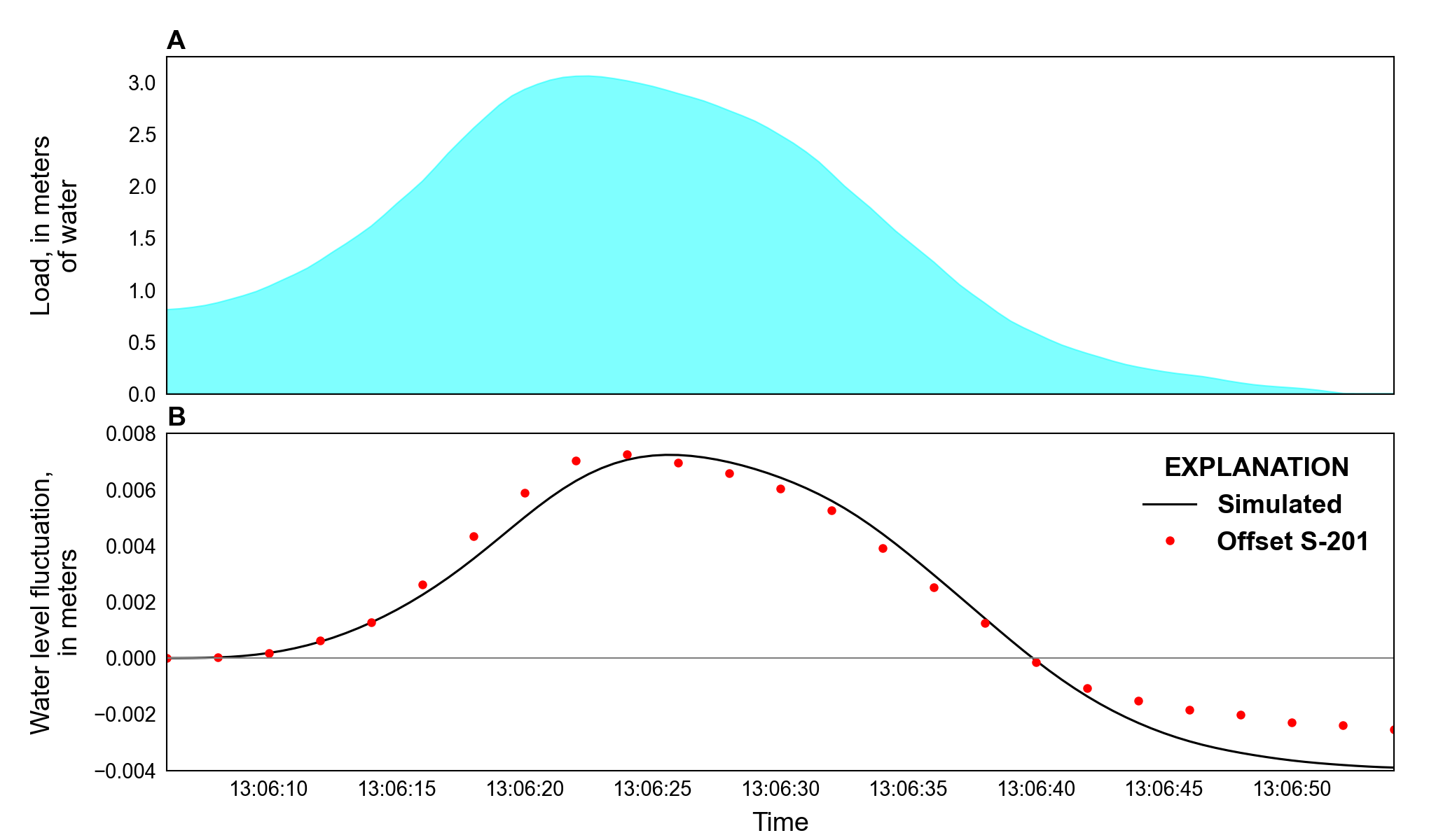
Figure 26.2 Graphs showing the applied loading and water-level fluctuations for the elastic aquifer loading problem. A, shows the loading applied to the top of the first column in layer 1, and B, shows simulated and offset water-level fluctuations at well S-201
The water-level fluctuation data used to calibrate the hydraulic parameters was offset so that the initial water-level fluctuation reported (after rewinding the pen-carriage cable) corresponded to a zero value. The adjusted water-level at the end of the simulation period is less than zero since loading of the aquifer by the train was already occurring at the beginning of the data presented in (Jacob, 1939) (fig Figure 26.2B). The water-level fluctuation data was offset rather than extended because of uncertainties about the train velocity and acceleration prior to the simulation period.
PEST++ (Welter et al., 2015) was used to calibrate the horizontal hydraulic conductivity in layers 1 and 3, the vertical hydraulic conductivity in layer 2, and specific storage values in all model layers. The water-level fluctuation observations were weighted by \(\text{max} ( 0.01, h_i / \text{max(h)} )\) to force PEST++ to favor the peak water-level fluctuations. The water-level fluctuations were only sensitive to the hydraulic conductivity and specific storage of model layer 3; as a result, PEST++ only modified the hydraulic properties of layer 3. Final hydraulic properties used in the model are shown in Table 26.2.
26.2. Example Results
A comparison of simulated and observed water-level fluctuations is shown in Figure 26.2B. For this problem, the MODFLOW 6 solution does not show perfect agreement with the offset water-level fluctuations. The primary source of model error is likely due primarily to inaccuracies in the loading being applied in the model. Use of a two-dimensional cross-section model instead of a three-dimensional model may also be responsible for a portion of the model error shown in Figure 26.2B. Horizontal strain has also been found to be significant in close proximity pumping wells (the source of strain) and may also contribute to the model error (Burbey, 2001).
26.3. References Cited
Burbey, T. J. (2001). Storage coefficient revisited–Is purely vertical strain a good assumption? Groundwater, 39(3), 458–464. https://doi.org/10.1111/j.1745-6584.2001.tb02330.x
Freeze, R. A., & Cherry, J. A. (1979). Groundwater (p. 604). Englewood Cliffs, N.J.: Prentice-Hall.
Jacob, C. (1939). Fluctuations in artesian pressure produced by passing railroad-trains as shown in a well on Long Island, New York. Eos, Transactions American Geophysical Union, 20(4), 666–674. https://doi.org/10.1029/TR020i004p00666
Welter, D. E., White, J. T., Hunt, R. J., & Doherty, J. E. (2015). Approaches in highly parameterized inversion–PEST++ Version 3, a Parameter ESTimation and uncertainty analysis software suite optimized for large environmental models. Retrieved from https://doi.org/10.3133/tm7C12
26.4. Jupyter Notebook
The Jupyter notebook used to create the MODFLOW 6 input files for this example and post-process the results is: