29. One-Dimensional Compaction in a Three-Dimensional Flow Field
This problem is based on the problem presented in the SUB-WT report (Leake & Galloway, 2007) and represent groundwater development in a hypothetical aquifer that includes some features typical of basin-fill aquifers in an arid or semi-arid environment. The problem of (Leake & Galloway, 2007) was modified to include compaction of coarse-grained aquifer materials and water compressibility. Specific stress packages were also modified but net inflows to the model domain are identical.
29.1. Example Description
The model grid for this problem consists of four layers, 20 rows, and 15 columns (Figure 29.1). The model has a top elevation of 150 meters and layer bottom elevations of 50, -100, -150, and -350 meters for layers 1, 2, 3, and 4, respectively. DELR and DELC are specified with a constant value of 2,000 meters. The simulation consists of three stress periods. The first is an initial steady-state period for the purpose of computing the head distribution, which is used with other quantities to compute the initial hydrostatic, effective, geostatic, and preconsolidation stresses. The second stress period is used to simulate 60 years of pumping by the two wells at locations shown in Figure 29.1. The third stress period is used to simulate 60 years of recovery following cessation of pumping. The second and third stress periods are divided into 60, 1-year time steps.
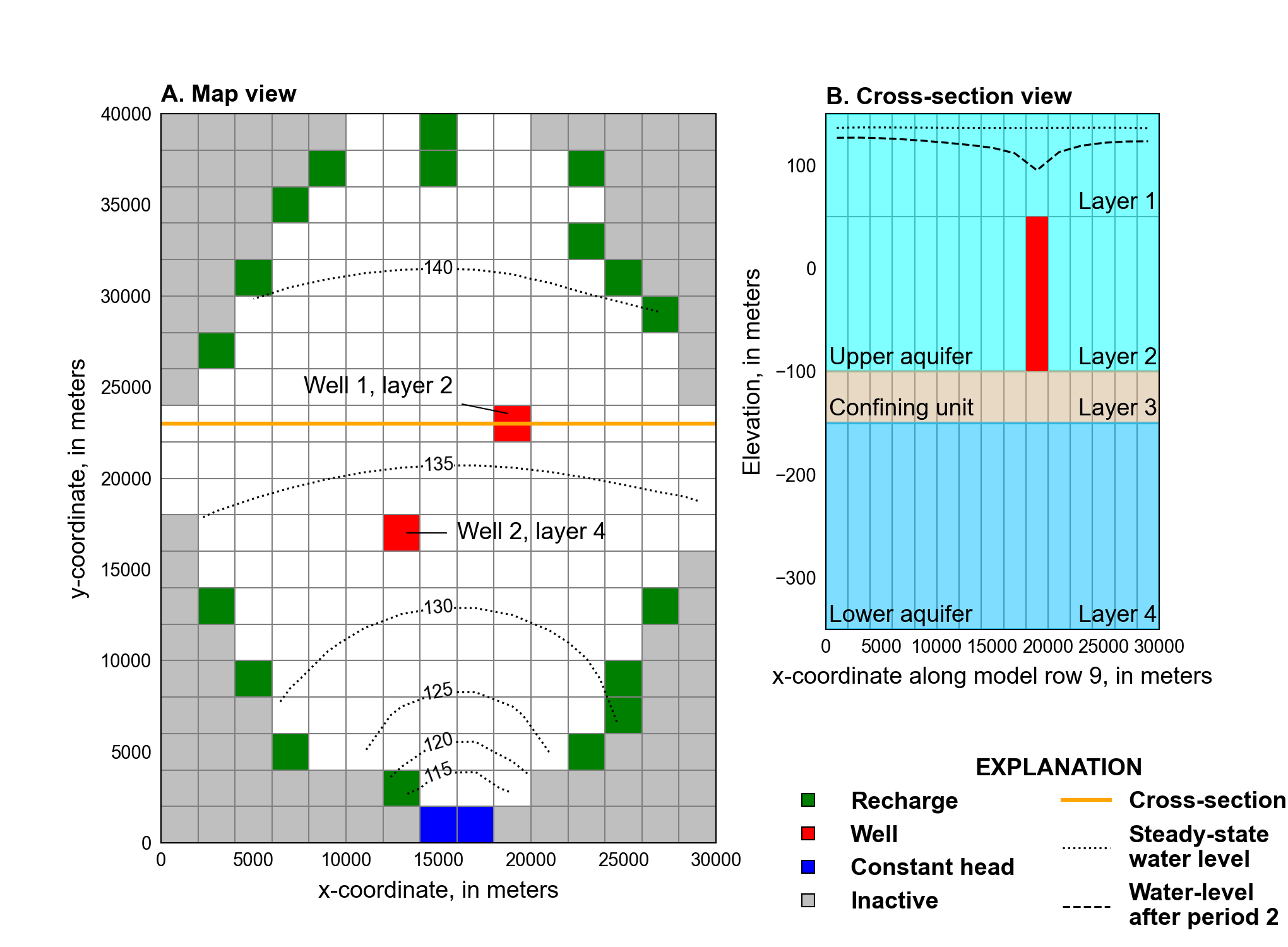
Figure 29.1 Diagram showing the model domain for the one-dimensional compaction in a three-dimensional flow field problem. A, plan view, and B, cross-section view. The locations of active and inactive areas of the model domain, steady-state heads in model layer 1, and locations of recharge cells, constant-head cells, and wells are also shown
The aquifer system consists of an unconfined upper aquifer, an extensive confining unit, and a confined lower aquifer (Figure 29.1B). The model uses two layers to represent the water-table aquifer and one layer each to represent the confining unit and the lower aquifer. Hydraulic conductivity was assumed to be isotropic in the horizontal and vertical directions in each layer. Hydraulic properties for coarse-grained materials are listed in Table 29.1. The specific storage was defined to be 0 for all layers in the STO package. Model layer 1 and layers 2–4 were defined to be convertible and non-convertible, respectively, for hydraulic conductivity and storage properties. Default NPF and STO package settings were used. An initial head of 100 meters was defined for each layer.
Parameter |
Value |
|---|---|
Number of periods |
3 |
Number of layers |
4 |
Number of rows |
20 |
Number of columns |
15 |
Column width (\(m\)) |
2000.0 |
Row width (\(m\)) |
2000.0 |
Top of the model (\(ft\)) |
150.0 |
Layer bottom elevations (\(m\)) |
50., –100., –150., –350. |
Starting head (\(m\)) |
100.0 |
Cell conversion type |
1, 0, 0, 0 |
Horizontal hydraulic conductivity (\(m/d\)) |
4., 4., 0.01, 4. |
Vertical hydraulic conductivity (\(m/d\)) |
0.4, 0.4, 0.01, 0.4 |
Specific yield (unitless) |
0.3, 0.3, 0.4, 0.3 |
Compressibility of water (Newtons/(\(m^3\)) |
9806.65 |
Specific gravity of water (1/\(Pa\)) |
4.6612e-10 |
Specific gravity of moist soils (unitless) |
1.77, 1.77, 1.60, 1.77 |
Specific gravity of saturated soils (unitless) |
2.06, 2.05, 1.94, 2.06 |
Coarse-grained material porosity (unitless) |
0.32, 0.32, 0.45, 0.32 |
Elastic specific storage (\(1/m\)) |
0.005, 0.005, 0.01, 0.005 |
Interbed thickness (\(m\)) |
45., 70., 50., 90. |
Interbed initial porosity (unitless) |
0.45 |
Interbed recompression index (unitless) |
0.01 |
Interbed compression index (unitless) |
0.25 |
Initial preconsolidation stress offset (\(m\)) |
15.0 |
The effective stress formulation of the CSUB package was used to simulate compaction of aquifer materials. Storage properties for coarse- and fine-grained materials were specified using compression indices. No-delay interbeds were specified in each active model cell. Hydraulic properties for fine-grained materials represented as no-delay interbeds are listed in Table 29.1; no-delay interbeds in model 3 comprise the full thickness of the confining unit.
The specific gravity of fully- and partially-saturated materials for each layer was calculated using
where \(G\) is the specific gravity of a control volume that includes solids and water (unitless), \(\bar{\theta}\) is the thickness weighted porosity of coarse- and fine-grained materials in a control volume (unitless), \(G_{\text{solid}}\) is the specific gravity of the solids in a control volume (unitless), \(k_r\) is a scaling factor used to scale the specific gravity of water if a control volume is not fully saturated (unitless), and \(G_{\text{water}}\) is the specific gravity of water (unitless). \(k_r\) is 1 for saturated materials or the ratio of the volume of water to the total volume for materials that are not fully saturated.
The specific gravity of saturated materials for each layer was calculated using the thickness weighted porosity listed in Table 29.1, a \(G_{\text{solid}}\) value of 2.7, and a \(G_{\text{water}}\) value of 1.0. The specific gravity of moist materials was calculated using a \(k_r\) value of 0.25 and the other values used to calculated the specific gravity of saturated materials. The specific gravity of saturated and moist materials used for the one-dimensional compaction in a three-dimensional flow field problem are listed in Table 29.1
Water compressibility was simulated and default specific gravity of water (\(\gamma_{\text{water}}\) = 4.6512 × 10⁻¹⁰ per Pascal) and the compressibility of water (\(\beta\) = 9806.65 Newtons per cubic meter) values were used. Initial specific storage values related to the compressibility of water (\(S_{s_{\text{water}}} = \theta \beta \gamma_{\text{water}}\)) were 1.46 × 10⁻⁶ and 2.05 × 10⁻⁶ per meter for coarse- and fine-grained materials, respectively. The porosity and thickness of coarse- and fine-grained materials were adjusted during the simulation in response to compaction. The initial preconsolidation stress for the no-delay interbeds was specified to be 15 meters greater than the steady-state effective stress calculated in each cell at the end of stress period 1.
Inflow to the flow system is simulated using the recharge package at 18 recharge locations in layer 1 shown on Figure 29.1A. Recharge at each of these locations is specified at a rate of 5.5 × 10⁻⁴ meters per day throughout the entire simulation, resulting in a total recharge rate of 39,600 cubic meters per day. Under steady-state conditions, all of the flow leaves the system through eight constant-head cells, two of which are in each layer at the horizontal locations shown on Figure 29.1A. Head at the eight constant-head cells is specified to be 100 meters. During stress period 2, each of the two wells shown on Figure 29.1A withdraw water from the upper and lower aquifer at a rate of 72,000 cubic meters per day.
29.2. Example Results
The initial steady-state stress period results in a maximum head of 143.0 meters in row 1, column 8. Steady-state hydraulic gradients slope down valley and toward the center of the valley to the constant-head cells in row 20, layers 1–4 (Figure 29.1). The steady-state head distribution is used to compute initial effective stress, preconsolidation stress, and geostatic stress for the transient part of the simulation. For the location of the well in row 9, column 10, layer 2, these stress values are 273.3, 288.3, and 509.5 meters, respectively.
Equivalent skeletal specific storage values were calculated from recompression and compression indices and the initial effective stress distribution. Computed values of elastic skeletal specific storage at row 9, column 10, were 2.03 × 10⁻⁵, 8.58 × 10⁻⁶, 7.33 × 10⁻⁶, and 4.41 × 10⁻⁶ per meter for layers 1–4, respectively. Values of inelastic (virgin) skeletal specific storage for the same location were 2.03 × 10⁻⁴, 8.58 × 10⁻⁵, 7.33 × 10⁻⁵, and 4.41 × 10⁻⁵ per meter for layers 1–4, respectively. These values are not used explicitly in further calculations by the CSUB package, but are provided to illustrate how effective stress influences the spatial distribution of specific storage.
29.2.1. Simulated Stresses
Values of effective stress, preconsolidation stress, and geostatic stress at the bottom of the cell for the 60-year pumping and 60-year recovery periods are shown in Figure 29.2 for row 9, column 10, layers 1 and 2. In both layers, preconsolidation stress is exceeded early in the simulation and tracks with increases in effective stress until recovery of water levels after the start of stress period 3 (year 60). Head change at this location is similar in layers 1 and 2, and the shapes and magnitudes of change-of-effective- and preconsolidation-stress curves are nearly the same (figs. Figure 29.2A, C). The curves, however, are at different head elevations because of the increase in magnitude of stress with depth. The shapes of curves representing geostatic stress in layers 1 and 2 (figs. Figure 29.2B, D) are identical because all of the change results from movement of the water table in layer 1 (Figure 29.1B). Note how simulated effective stress and geostatic stress does not return to initial values 60 years after cessation of pumpage; approximately 2,000 years without pumping is required for simulated effective stress and geostatic stress at row 9, column 10, layers 1 and 2 to return initial values.
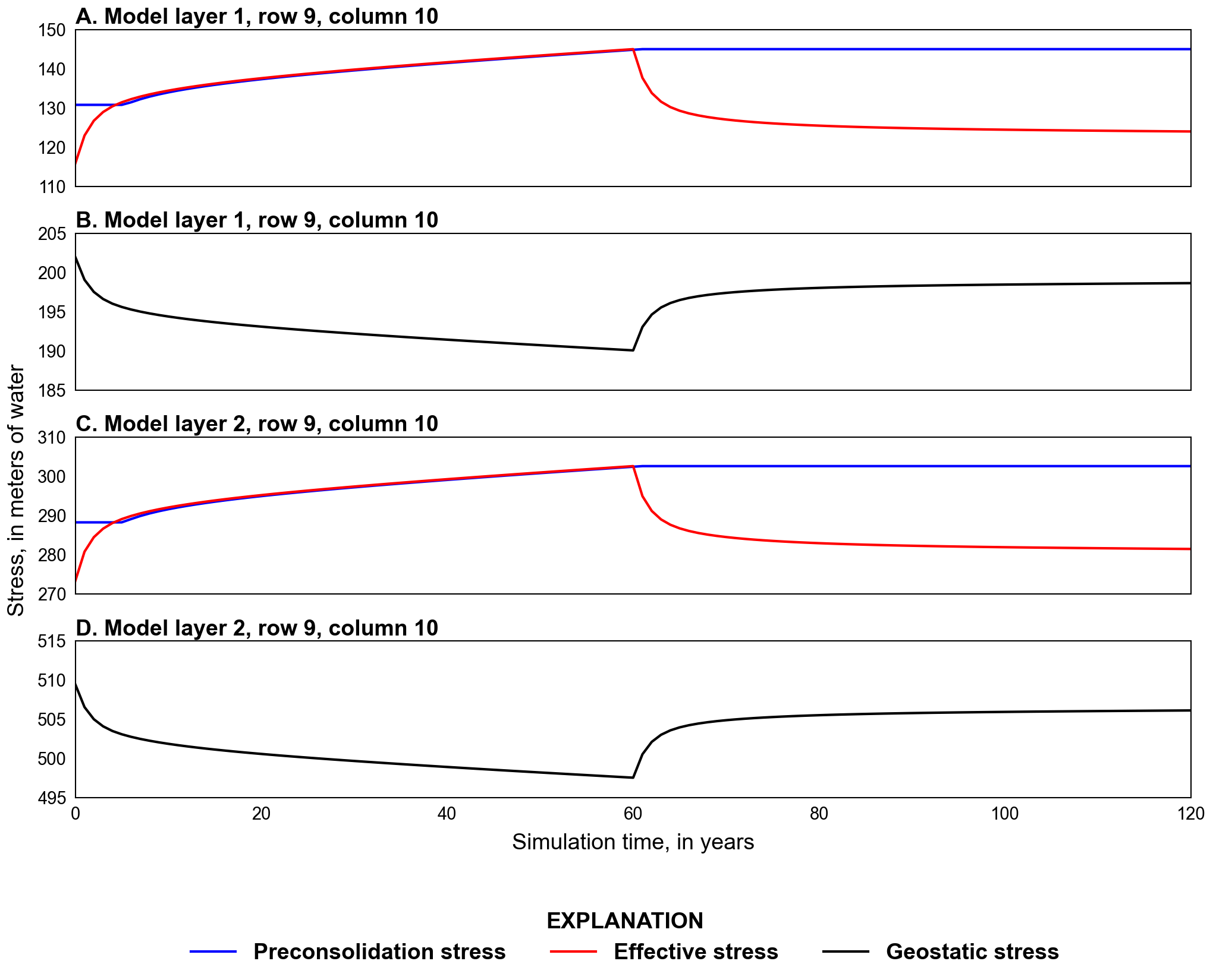
Figure 29.2 Graphs showing computed stresses for row 9, column 10 for the one-dimensional compaction in a three-dimensional flow field problem. A, Effective and preconsolidation stress in layer 1, B, geostatic stress in layer 1, C, effective and preconsolidation stress in layer 2, and D, geostatic stress in layer 2
29.2.2. Simulated Compaction
The computed vertical displacements for the tops of layers 1–4 resulting from fine- (interbed) and coarse-grained material compaction at the locations of the two pumping wells are shown in Figure 29.3. The total compaction at the top of layer 1 represent the time series of land subsidence for the two locations (Figure 29.3E, F). Similarly, differences between displacement curves for adjacent layers are the time distributions of compaction in the each layer. At both locations, compaction is greatest in the layer in which pumping takes place. Coarse-grained compaction is small relative to inelastic compaction of fine-grained interbeds. Similar to stress results (Figure 29.2), elastic compaction of coarse-grained materials does not fully recover 60 years after cessation of pumpage.
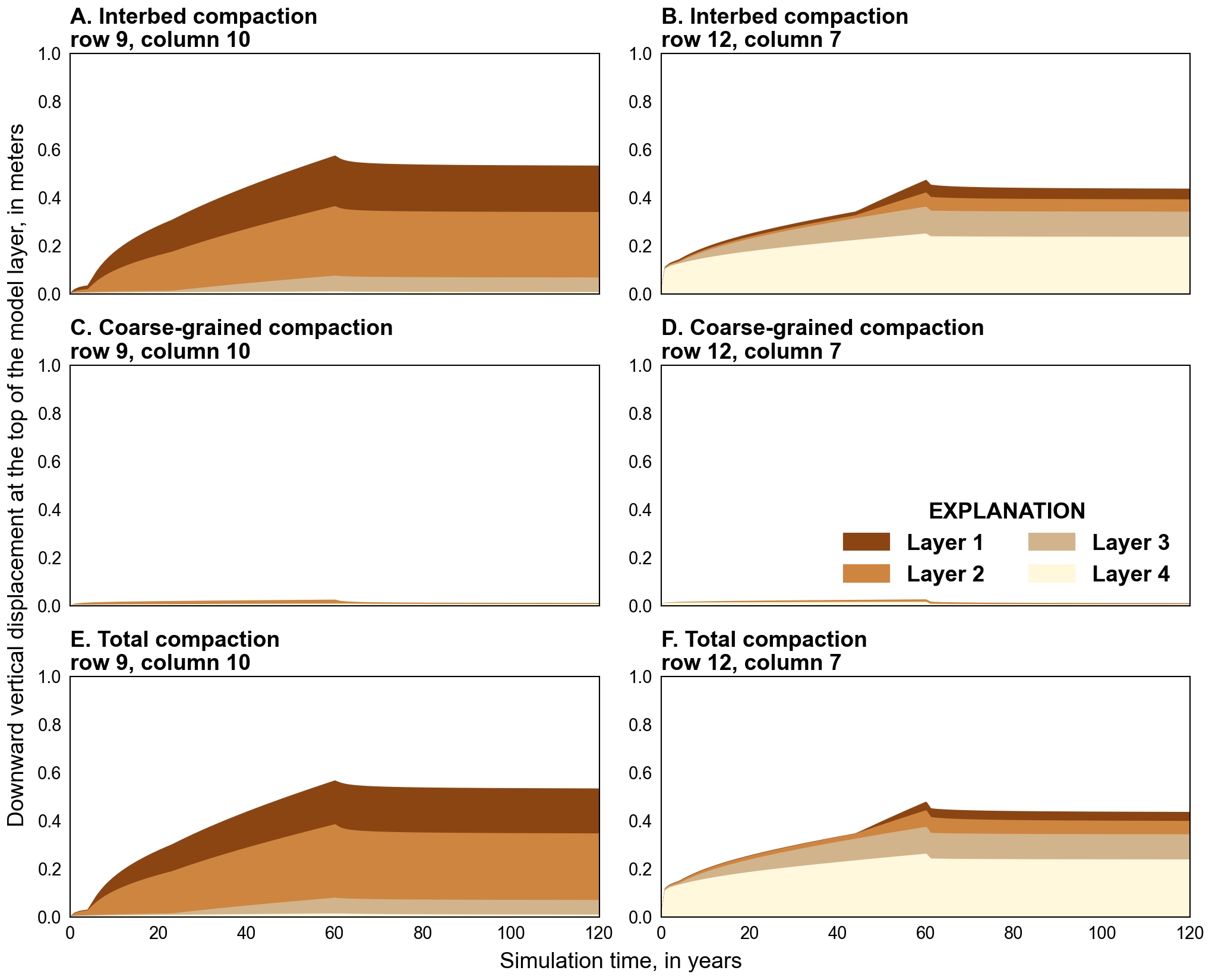
Figure 29.3 Graphs showing computed downward displacement for the tops of model layers 1–4 for the one-dimensional compaction in a three-dimensional flow field problem. A, interbed compaction at row 9, column 10, B, interbed compaction at row 12, column 7, C, coarse-grained material compaction at row 9, column 10, D, coarse-grained material compaction at row 12, column 7, E, total compaction at row 9, column 10, and F, total compaction at row 12, column 7
29.2.3. Simulated Storage Changes
At the end of the second stress period a total of 3,155,760,128 cubic meters of water was pumped from the water-table and confined aquifers. Water released from specific yield, elastic coarse-grained materials, elastic fine-grained materials, inelastic fine-grained materials, and water compressibility accounted for 96.31% (3,039,304,920 cubic meters) of groundwater pumpage; the remainder of groundwater pumpage came from reduction in the discharge to the eight constant-head cells. Individually specific yield, elastic coarse-grained materials, elastic fine-grained materials, inelastic fine-grained materials, and water compressibility accounted for 94.80%, 0.40%, 0.63%, 0.21%, and 0.27%, respectively, of total groundwater pumpage. For the cell containing well 1 (layer 2, row 9, column 10) elastic coarse-grained materials, elastic fine-grained materials, inelastic fine-grained materials, and water compressibility accounted for 5.18%, 3.81%, 87.68%, and 3.33%, respectively, of the total water released from storage (3,628.59 cubic meters) in response to groundwater pumpage. For the cell containing well 2 (layer 4, row 12, column 7) elastic coarse-grained materials, elastic fine-grained materials, inelastic fine-grained materials, and water compressibility accounted for 4.63%, 2.62%, 87.57%, and 5.18%, respectively, of the total water released from storage (3,147.01 cubic meters) in response to groundwater pumpage.
29.3. References Cited
Leake, S. A., & Galloway, D. L. (2007). MODFLOW Ground-water model—User guide to the Subsidence and Aquifer-System Compaction Package (SUB-WT) for Water-Table Aquifers. Retrieved from https://pubs.er.usgs.gov/publication/tm6A23
29.4. Jupyter Notebook
The Jupyter notebook used to create the MODFLOW 6 input files for this example and post-process the results is: