34. MOC3D Problem 1
This problem corresponds to the first problem presented in the MOC3D report (Konikow et al., 1996), which involves the transport of a dissolved constituent in a steady, one-dimensional flow field. An analytical solution for this problem is given by (Wexler, 1992). This example is simulated with the GWT Model in MODFLOW 6, which receives flow information from a separate simulation with the GWF Model in MODFLOW 6. Results from the GWT Model are compared with the results from the (Wexler, 1992) analytical solution.
34.1. Example description
The parameters used for this problem are listed in Table 34.1. The model grid for this problem consists of one layer, 120 rows, and 1 columns. The top for each cell is assigned a value of 1.0 \(cm\) and the bottom is assigned a value of zero. DELR is set to 1.0 \(cm\) and DELC is specified with a constant value of 0.1 \(cm\). The simulation consists of one stress period that is 120 \(s\) in length, and the stress period is divided into 240 equally sized time steps. By using a uniform porosity value of 0.1, a velocity value of 0.1 \(cm/s\) results from the injection of water at a rate of 0.001 \(cm^3/s\) into the first cell. The last cell is assigned a constant head with a value of zero, though this value is not important as the cells are marked as being confined. The concentration of the injected water is assigned a value of 1.0, and any water that leaves through the constant-head cell leaves with the simulated concentration of the water in that last cell. Advection is solved using the TVD scheme to reduce numerical dispersion.
Parameter |
Value |
|---|---|
Number of periods |
1 |
Number of layers |
1 |
Number of rows |
1 |
Number of columns |
122 |
Length of system (\(cm\)) |
12.0 |
Column width (\(cm\)) |
0.1 |
Row width (\(cm\)) |
0.1 |
Top of the model (\(cm\)) |
1.0 |
Layer bottom elevation (\(cm\)) |
0 |
Specific discharge (\(cm s^{-1}\)) |
0.1 |
Hydraulic conductivity (\(cm s^{-1}\)) |
0.01 |
Porosity of mobile domain (unitless) |
0.1 |
Simulation time (\(s\)) |
120.0 |
Source concentration (unitless) |
1.0 |
Initial concentration (unitless) |
0.0 |
34.2. Example Scenarios
This example problem consists of several different scenarios, as listed in Table 34.2. Two different levels of dispersion were simulated, and these simulations are referred to as the low dispersion case and the high dispersion case. The low dispersion case has a dispersion coefficient of 0.01 \(cm^2/s\), which, for the specified velocity, corresponds to a dispersivity value of 0.1 \(cm\). The high-dispersion case has a dispersion coefficient of 0.1 \(cm^2/s\), which corresponds to a dispersivity value of 1.0 \(cm\).
Scenario |
Scenario Name |
Parameter |
Value |
|---|---|---|---|
1 |
ex-gwt-moc3d-p01a |
longitud inal dispersivity (\(cm\)) |
0.1 |
r etardation factor (unitless) |
1.0 |
||
decay rate (\(s^{-1}\)) |
0.0 |
||
2 |
ex-gwt-moc3d-p01b |
longitud inal dispersivity (\(cm\)) |
1.0 |
r etardation factor (unitless) |
1.0 |
||
decay rate (\(s^{-1}\)) |
0.0 |
||
3 |
ex-gwt-moc3d-p01c |
longitud inal dispersivity (\(cm\)) |
1.0 |
r etardation factor (unitless) |
2.0 |
||
decay rate (\(s^{-1}\)) |
0.0 |
||
4 |
ex-gwt-moc3d-p01d |
longitud inal dispersivity (\(cm\)) |
1.0 |
r etardation factor (unitless) |
1.0 |
||
decay rate (\(s^{-1}\)) |
0.01 |
34.2.1. Scenario Results
For the first scenario with a relatively small dispersivity value (0.1 \(cm\)), plots of concentration versus time and concentration versus distance are shown in Figure 34.1 and
Figure 34.2, respectively.
Figure 34.1 can be compared to figure 18 in (Konikow et al., 1996). The three separate concentration versus time curves represent the three different distances (0.05, 4.05, and 11.05 cm). For this low-dispersion case, the MODFLOW 6 solution is in relatively good agreement with the analytical solution, but some slight differences are observed. These differences are due primarily to limitations with the second-order TVD scheme implemented in MODFLOW 6, which can suffer from numerical dispersion.
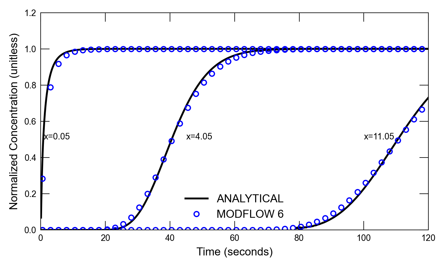
Figure 34.1 Concentrations simulated by the MODFLOW 6 GWT Model and calculated by the analytical solution for one-dimensional flow with transport for the low dispersion case. Circles are for the GWT Model results; the lines represent the analytical solution by (Wexler, 1992). Results are shown for three different distances (0.05, 4.05, and 11.05 \(cm\) from the end of the first cell). Every fifth time step is shown for the MODFLOW 6 results.
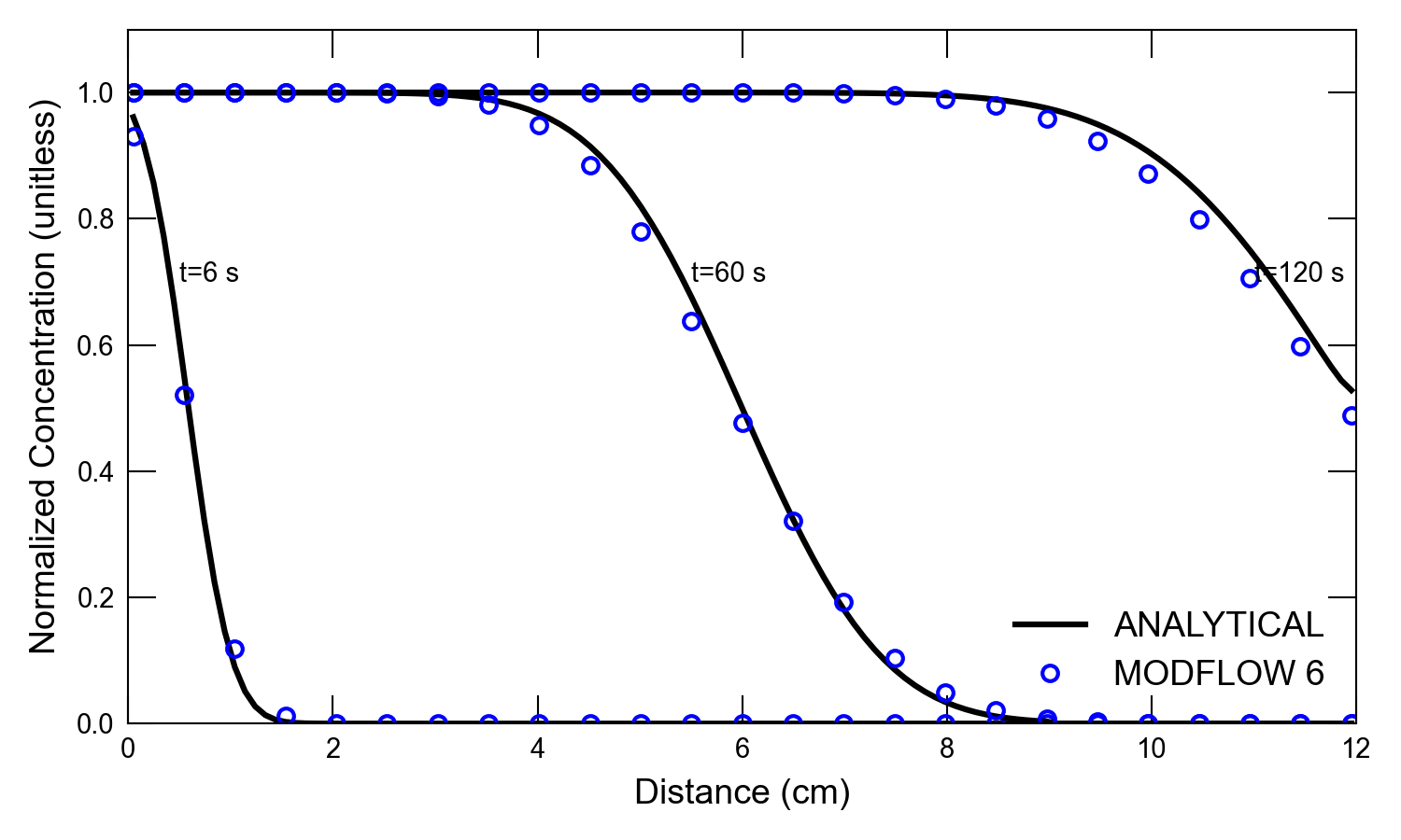
Figure 34.2 Concentrations simulated by the MODFLOW 6 GWT Model and calculated by the analytical solution for one-dimensional flow with transport for the low dispersion case. Circles are for the GWT Model results; the lines represent the analytical solution by (Wexler, 1992). Results are shown for three different times (6, 60, and 120 \(s\)). Every fifth cell is shown for the MODFLOW 6 results.
For the second scenario, which has a relatively large dispersivity value (1.0 \(cm\)), plots of concentration versus time and concentration versus distance are shown in Figure 34.3 and Figure 34.4, respectively. For the high-dispersion case, the results from the MODFLOW 6 simulation are in better agreement with the analytical solution than for the low dispersion case.
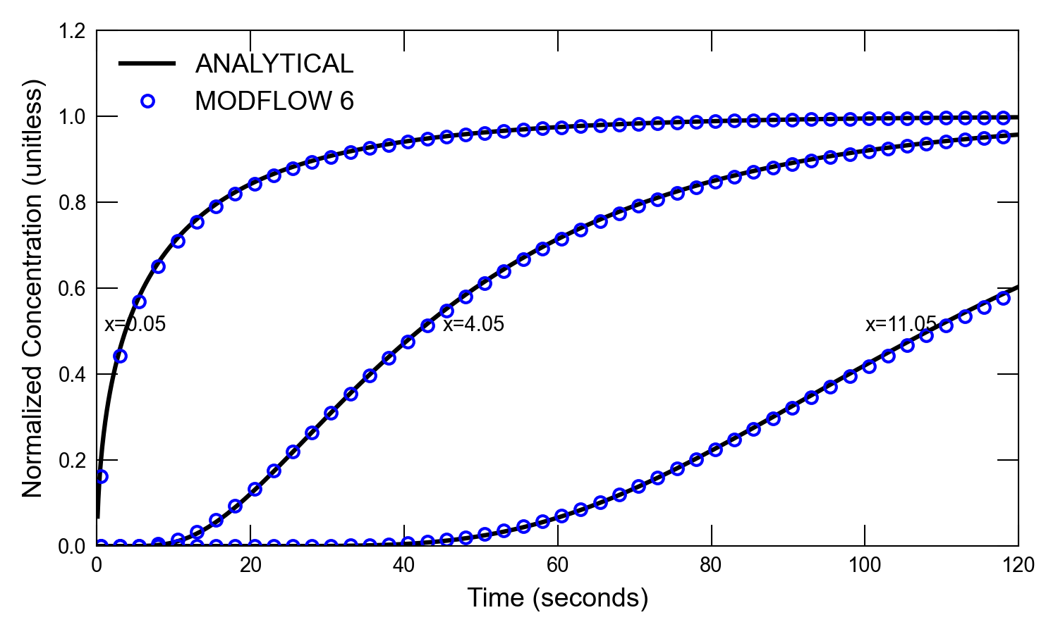
Figure 34.3 Concentrations simulated by the MODFLOW 6 GWT Model and calculated by the analytical solution for one-dimensional flow with transport for the high dispersion case. Circles are for the GWT Model results; the lines represent the analytical solution by (Wexler, 1992). Results are shown for three different distances (0.05, 4.05, and 11.05 \(cm\) from the end of the first cell). Every fifth time step is shown for the MODFLOW 6 results.
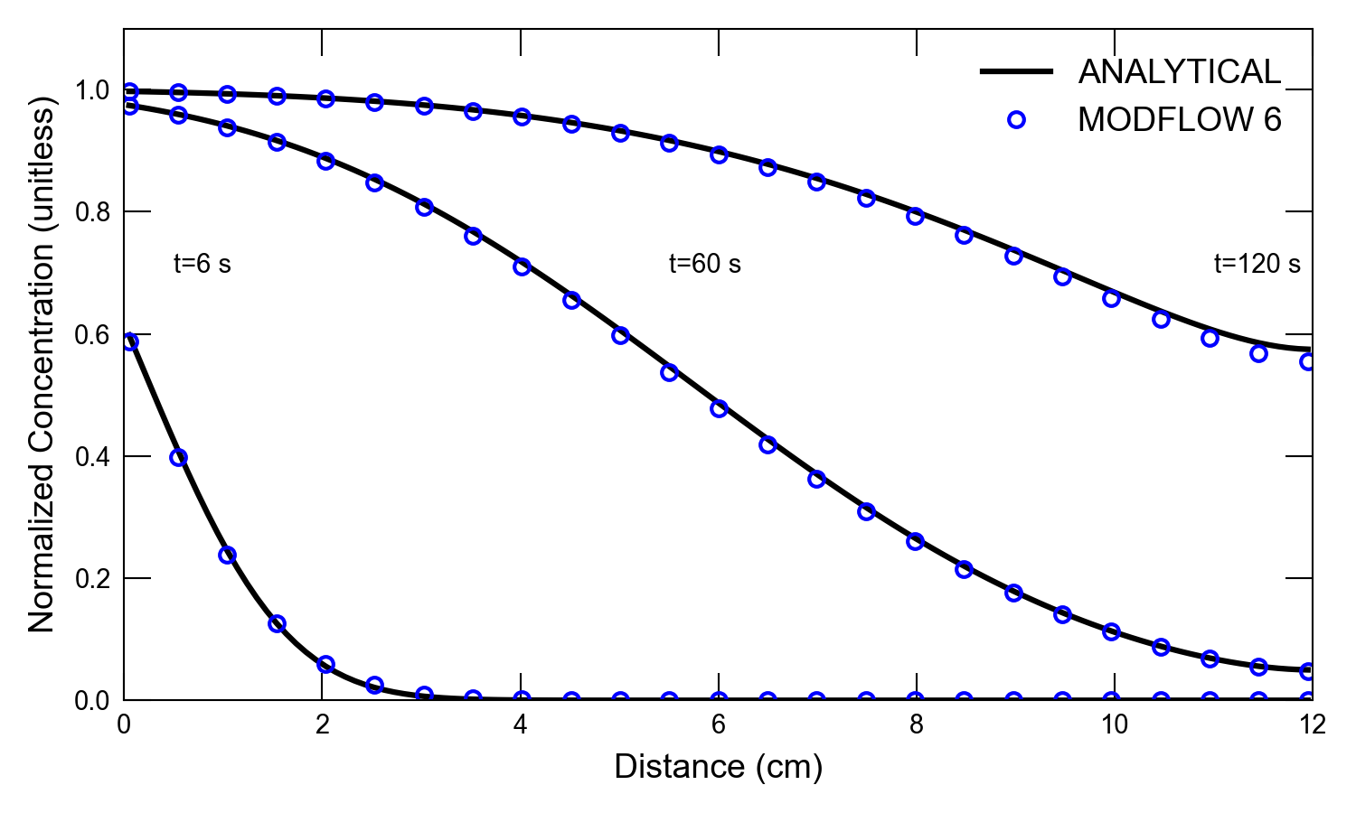
Figure 34.4 Concentrations simulated by the MODFLOW 6 GWT Model and calculated by the analytical solution for one-dimensional flow with transport for the high dispersion case. Circles are for the GWT Model results; the lines represent the analytical solution by (Wexler, 1992). Results are shown for three different times (6, 60, and 120 \(s\)). Every fifth cell is shown for the MODFLOW 6 results.
For the remaining scenarios, the results from MODFLOW 6 are compared with the (Wexler, 1992) analytical solution for two variations of the high-dispersion case. The effects sorption are included in scenario 3 and the effects of decay are included in scenario 4. Plots of concentration versus time and concentration versus distance for a simulation with a retardation factor of 2.0 are shown in Figure 34.5 and
Figure 34.6, respectively. Plots of concentration
versus time and concentration versus distance for a simulation with a decay rate of 0.01 \(s^{-1}\) are shown in Figure 34.7 and
Figure 34.8, respectively.
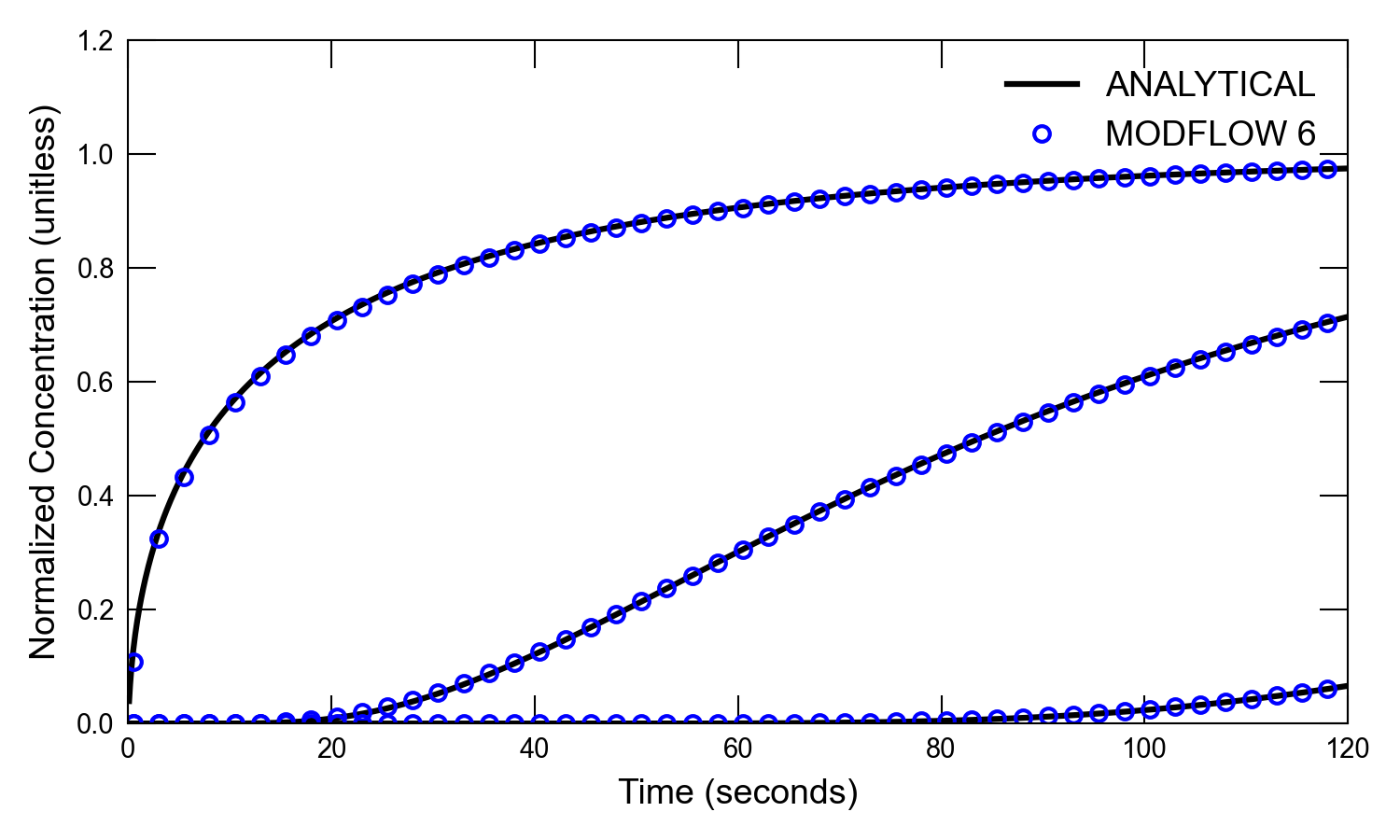
Figure 34.5 Concentrations simulated by the MODFLOW 6 GWT Model and calculated by the analytical solution for one-dimensional flow with transport for the high dispersion case and a retardation factor of 2. Circles are for the GWT Model results; the lines represent the analytical solution by (Wexler, 1992). Results are shown for three different distances (0.05, 4.05, and 11.05 \(cm\) from the end of the first cell). Every fifth time step is shown for the MODFLOW 6 results.
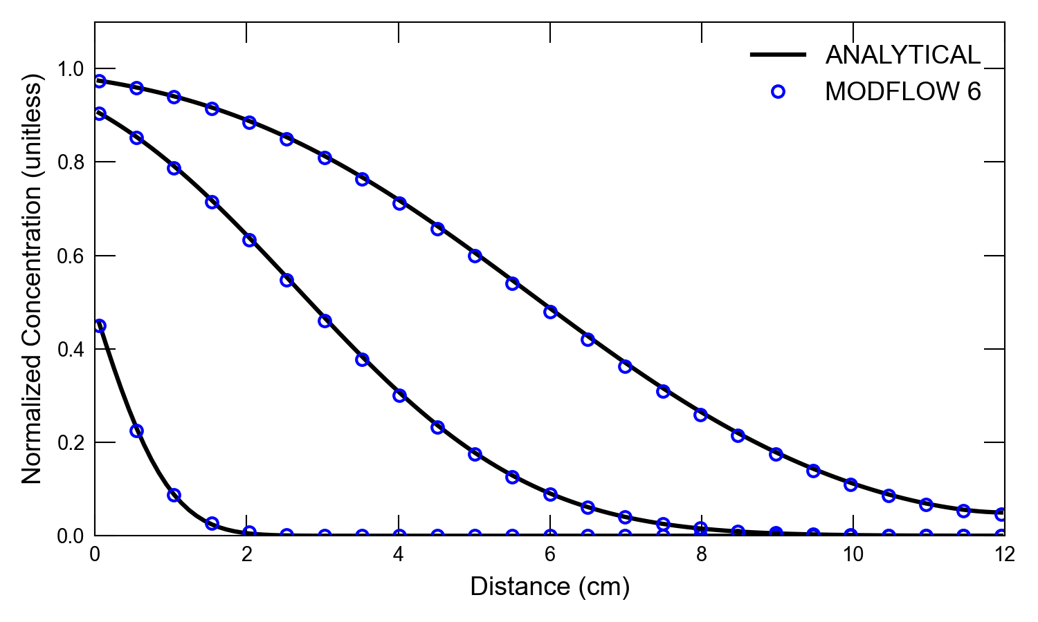
Figure 34.6 Concentrations simulated by the MODFLOW 6 GWT Model and calculated by the analytical solution for one-dimensional flow with transport for the high dispersion case and a retardation factor of 2. Circles are for the GWT Model results; the lines represent the analytical solution by (Wexler, 1992). Results are shown for three different times (6, 60, and 120 \(s\)). Every fifth cell is shown for the MODFLOW 6 results.
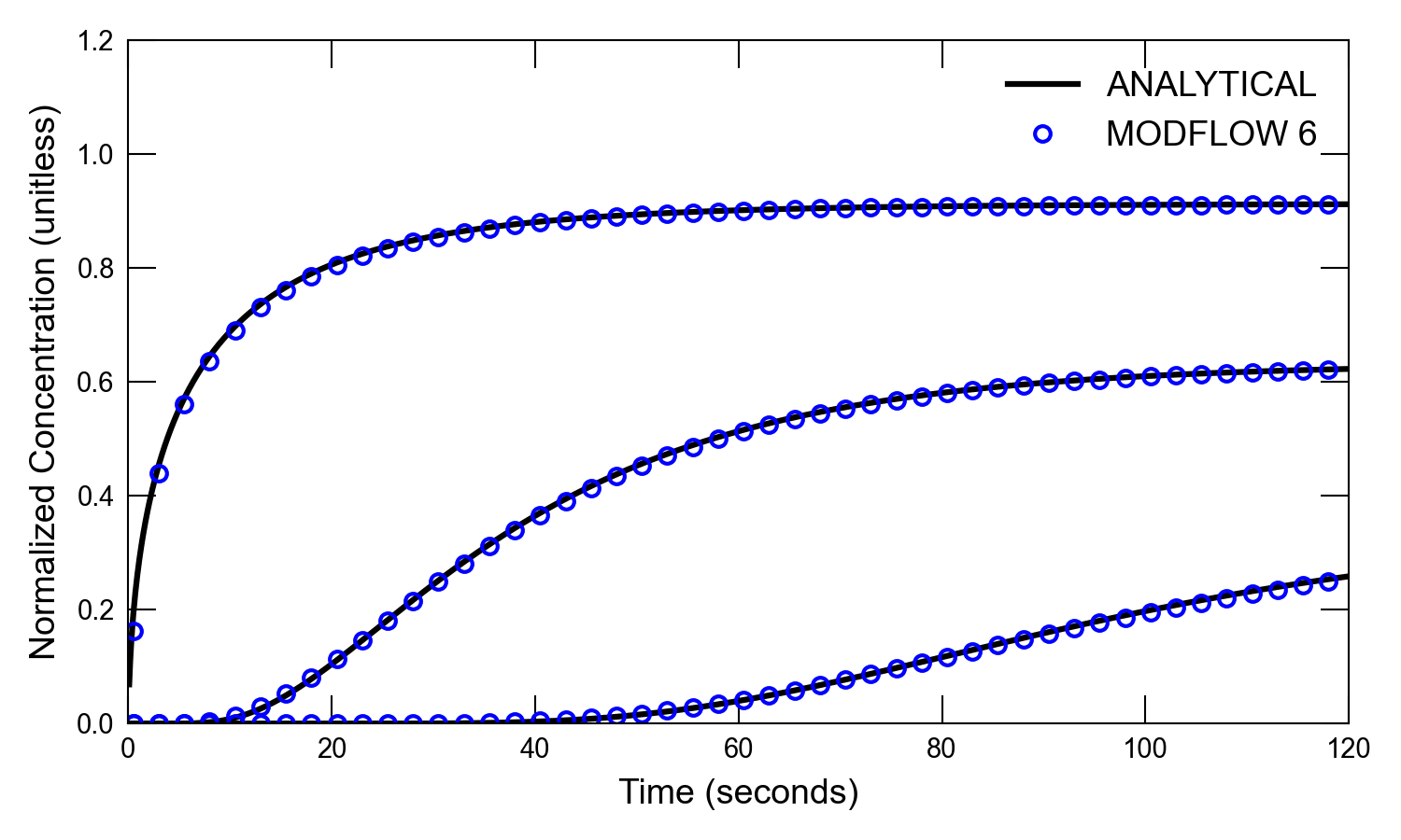
Figure 34.7 Concentrations simulated by the MODFLOW 6 GWT Model and calculated by the analytical solution for one-dimensional flow with transport for the high dispersion case and a decay rate of 0.01 \(s^{-1}\). Circles are for the GWT Model results; the lines represent the analytical solution by (Wexler, 1992). Results are shown for three different distances (0.05, 4.05, and 11.05 \(cm\) from the end of the first cell). Every fifth time step is shown for the MODFLOW 6 results.
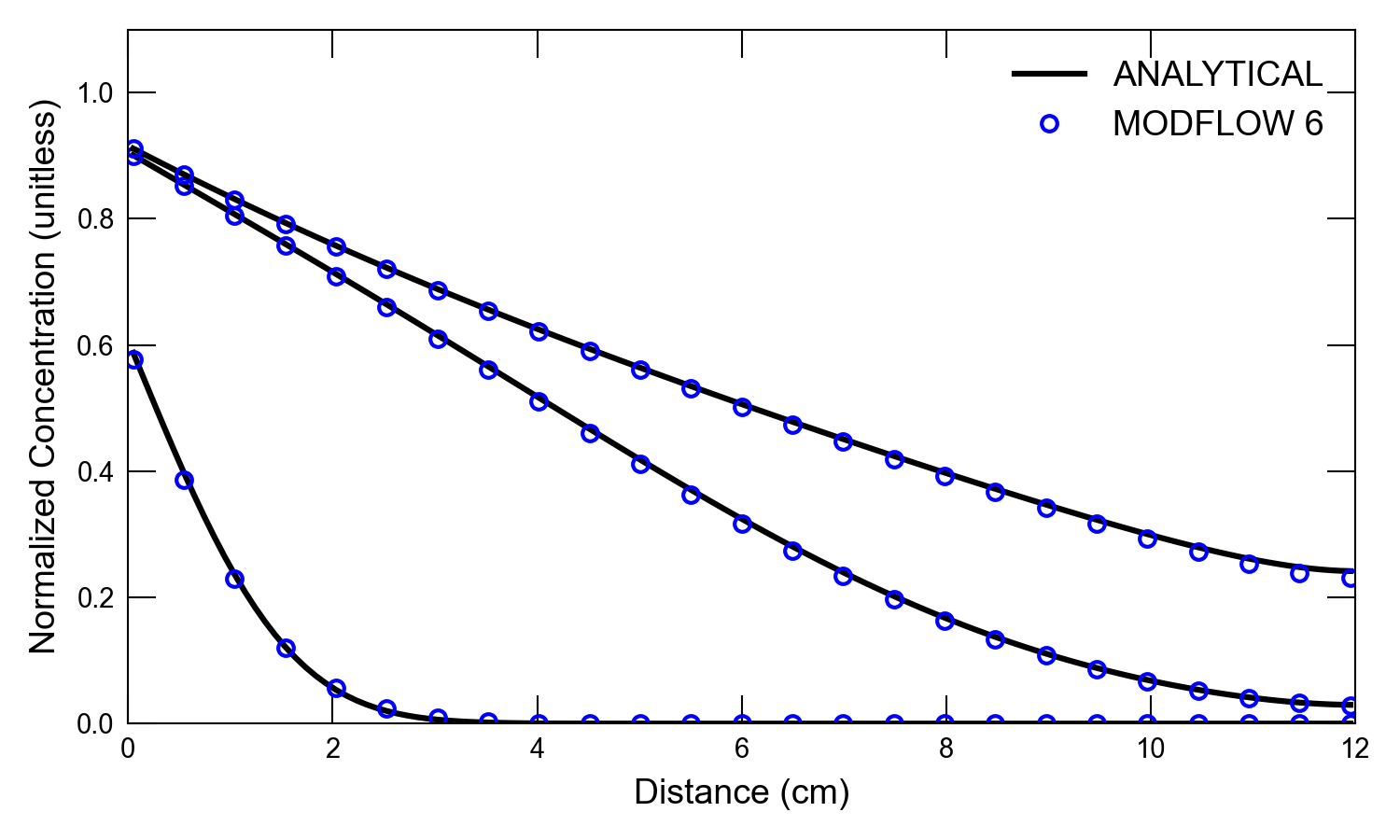
Figure 34.8 Concentrations simulated by the MODFLOW 6 GWT Model and calculated by the analytical solution for one-dimensional flow with transport for the high dispersion case and a decay rate of 0.01 \(s^{-1}\). Circles are for the GWT Model results; the lines represent the analytical solution by (Wexler, 1992). Results are shown for three different times (6, 60, and 120 \(s\)). Every fifth cell is shown for the MODFLOW 6 results.
34.3. References Cited
Konikow, L. F., Goode, D. J., & Hornberger, G. Z. (1996). A three-dimensional method-of-characteristics solute-transport model (MOC3D). Retrieved from https://pubs.er.usgs.gov/publication/wri964267
Wexler, E. J. (1992). Analytical solutions for one-, two-, and three-dimensional solute transport in ground-water systems with uniform flow.
34.4. Jupyter Notebook
The Jupyter notebook used to create the MODFLOW 6 input files for this example and post-process the results is: