38. MT3DMS Problem 2
This is the second example problem presented in (Zheng & Wang, 1999), titled “one-dimensional transport with nonlinear or nonequilibrium sorption.” The purpose of this example is to demonstrate simulation of nonlinear and nonequilibrium sorption. For the nonlinear sorption simulations, which use the Freundlich and Langmuir isotherms, (Zheng & Wang, 1999) compared MT3DMS results to the results from an independent transport simulator called CXTFIT. For the nonequilibrium sorption example, (Zheng & Wang, 1999) compared the results from MT3DMS to an analytical solution. In this section the results from the MODFLOW 6 GWT Model are compared with the results from MT3DMS.
In MT3DMS, nonequilibrium sorption is represented using the following expression for the dissolved and sorbed solute mass,
where \(\rho_b\) is the bulk density, \(\overline{C}\) is the sorbed concentration, \(C\) is the dissolved aqueous concentration, \(\beta\) is the first-order mass transfer rate between the dissolved aqueous and sorbed phases, \(t\) is time, and \(K_d\) is the linear distribution coefficient.
The current version of the MODFLOW 6 GWT Model does not have the capability to directly represent this type of nonequilibrium sorption. For the example presented by (Zheng & Wang, 1999), the distribution coefficient has a value close to one (0.933). Because this value is so close to one, we can take advantage of immobile domain capability in MODFLOW 6 to approximate nonequilibrium sorption. For this example there is no separate sorption process within the immobile domain, and there is no decay or production within the immobile domain (as has been defined for this example). Thus, for this problem the transfer of dissolved solute mass between the mobile and immobile domain can be expressed as
where \(\theta_{im}\) is the porosity of the immobile domain, \(\zeta\) is the first-order mass transfer rate between the mobile and immobile domains, and \(C_{im}\) is the concentration of the immobile domain. From the similar form of these two equations, it is possible to approximate the nonequilibrium sorption capability in MT3DMS by assigning the immobile domain porosity as bulk density and the first-order mass transfer rate for the mobile and immobile domain as the first-order mass transfer rate for the dissolved and sorbed phases.
There are six scenarios described here (table Table 38.1). The first two represent nonlinear sorption with the Freundlich and Langmuir isotherms, respectively. The remaining four scenarios represent nonequilibrium sorption with different values for the first-order mass transfer coefficient. These six scenarios and corresponding figures correspond to the ones reported by (Zheng & Wang, 1999).
Scenario |
Scenario Name |
Parameter |
Value |
|---|---|---|---|
1 |
e x-gwt-mt3dms-p02a |
sorption (text string) |
freundlich |
Kf (:math:`mu g
|
0.3 |
||
a (unitless) |
0.7 |
||
2 |
e x-gwt-mt3dms-p02b |
sorption (text string) |
langmuir |
Kl (: math:L mg^{-1}) |
100.0 |
||
S (:mat h:mu g g^{-1}) |
0.003 |
||
3 |
e x-gwt-mt3dms-p02c |
beta (\(s^{-1}\)) |
0.0 |
4 |
e x-gwt-mt3dms-p02d |
beta (\(s^{-1}\)) |
0.002 |
5 |
e x-gwt-mt3dms-p02e |
beta (\(s^{-1}\)) |
0.01 |
6 |
e x-gwt-mt3dms-p02f |
beta (\(s^{-1}\)) |
20.0 |
38.1. Example description
All model scenarios have 101 columns, 1 row, and 1 layer. The first column has a specified inflow rate that results in a velocity of 0.1 \(cm/s\). The last column is assigned as a constant-head boundary to allow water to exit. For the first 160 \(s\), a pulse of solute is introduced to the inflowing water. For the remaining 1340 \(s\), the concentration of inflowing water is zero. Additional model parameters are shown in Table 38.2.
Parameter |
Value |
|---|---|
Number of periods |
2 |
Number of layers |
1 |
Number of rows |
1 |
Number of columns |
101 |
Length of period 1 (\(s\)) |
160 |
Length of period 2 (\(s\)) |
1340 |
Length of time steps (\(s\)) |
1.0 |
Column width (\(cm\)) |
0.16 |
Row width (\(cm\)) |
0.16 |
Top of the model (\(cm\)) |
1.0 |
Layer bottom elevation (\(cm\)) |
0 |
Velocity (\(cm s^{-1}\)) |
0.1 |
Hydraulic conductivity (\(cm s^{-1}\)) |
0.01 |
Porosity of mobile domain (unitless) |
0.37 |
Bulk density (\(g cm^{-3}\)) |
1.587 |
Distribution coefficient (\(cm^3 g^{-1}\)) |
0.933 |
Longitudinal dispersivity (\(cm\)) |
1.0 |
Source concentration (unitless) |
0.05 |
Initial concentration (unitless) |
0.0 |
38.2. Example Results
Simulated results for nonlinear sorption are shown for the Freundlich isotherm in Figure 38.1 and for the Langmuir isotherm in Figure 38.2. The results from MODFLOW 6 compare well with the results from MT3DMS. Results for the four simulations with different values for beta are shown in Figure 38.3. For small beta values, the MODFLOW 6 results compare well with the results from MT3DMS. But for larger beta values, there are small discrepancies between the two models. This is because of the distribution coefficient value (0.933) used for the MT3DMS simulations and the approximation approach for the MODFLOW 6 simulation, which assumes the distribution coefficient is one. If a value of one is used for the distribution coefficient in the MT3DMS simulations, then results are virtually indistinguishable.
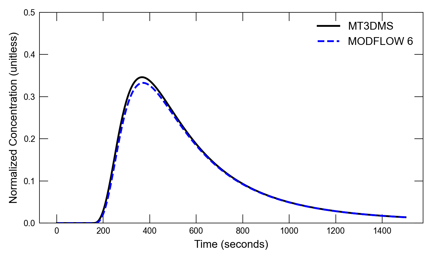
Figure 38.1 Comparison of the MT3DMS and MODFLOW 6 results for nonlinear sorption represented with the Freundlich isotherm.
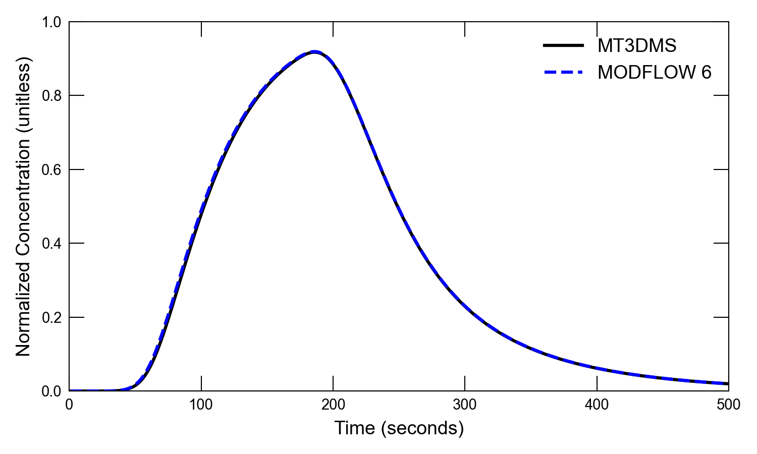
Figure 38.2 Comparison of the MT3DMS and MODFLOW 6 results for nonlinear sorption represented with the Langmuir isotherm.
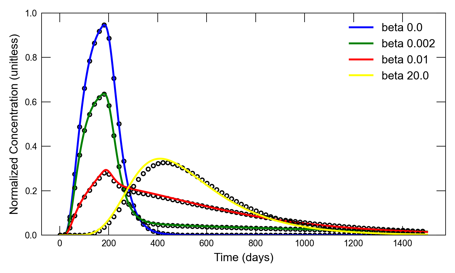
Figure 38.3 Comparison of the MT3DMS (solid lines) and MODFLOW 6(circles) results for four different values of the nonequilibrium exchange coefficient (beta). The results for MODFLOW 6 are shown for every 20th time step.
38.3. References Cited
Zheng, C., & Wang, P. P. (1999). MT3DMS—a modular three-dimensional multi-species transport model for simulation of advection, dispersion and chemical reactions of contaminants in groundwater systems; documentation and user’s guide.
38.4. Jupyter Notebook
The Jupyter notebook used to create the MODFLOW 6 input files for this example and post-process the results is: